Implementation of a UAV–Hyperspectral Pushbroom Imager for Ecological Monitoring

Abstract

Hyperspectral remote sensing provides a wealth of data essential for vegetation studies encompassing a wide range of applications (e.g., species diversity, ecosystem monitoring, etc.). The development and implementation of UAV-based hyperspectral systems have gained popularity over the last few years with novel efforts to demonstrate their operability. Here we describe the design, implementation, testing, and early results of the UAV-μCASI system, which showcases a relatively new hyperspectral sensor suitable for ecological studies. The μCASI (288 spectral bands) was integrated with a custom IMU-GNSS data recorder built in-house and mounted on a commercially available hexacopter platform with a gimbal to maximize system stability and minimize image distortion. We deployed the UAV-μCASI at three sites with different ecological characteristics across Canada: The Mer Bleue peatland, an abandoned agricultural field on Ile Grosbois, and the Cowichan Garry Oak Preserve meadow. We examined the attitude data from the flight controller to better understand airframe motion and the effectiveness of the integrated Differential Real Time Kinematic (RTK) GNSS. We describe important aspects of mission planning and show the effectiveness of a bundling adjustment to reduce boresight errors as well as the integration of a digital surface model for image geocorrection to account for parallax effects at the Mer Bleue test site. Finally, we assessed the quality of the radiometrically and atmospherically corrected imagery from the UAV-μCASI and found a close agreement (<2%) between the image derived reflectance and in-situ measurements. Overall, we found that a flight speed of 2.7 m/s, careful mission planning, and the integration of the bundling adjustment were important system characteristics for optimizing the image quality at an ultra-high spatial resolution (3–5 cm). Furthermore, environmental considerations such as wind speed (<5 m/s) and solar illumination also play a critical role in determining image quality. With the growing popularity of “turnkey” UAV-hyperspectral systems on the market, we demonstrate the basic requirements and technical challenges for these systems to be fully operational.

1. Introduction

The use of hyperspectral remote sensing in vegetation studies is well established for a wide array of ecosystems (e.g., [1,2,3,4,5]). Hundreds of contiguous spectral bands most commonly within the visible, near, and shortwave infrared regions of the electromagnetic spectrum (0.4–2.5 µm) provide detailed information on plant chemical and structural characteristics that are useful for species richness assessments (e.g., [2,6]), invasive species studies (e.g., [7,8]) and plant health (e.g., [9,10,11]). Absorption features related to photosynthetic pigments (e.g., chlorophyll) and other constituents (e.g., water and nitrogen) provide a unique make-up of the plant condition that is expressed by the vegetation spectral signature. Therefore, variations in shape and sometimes amplitude of the spectral signature can be used to, for example, identify individual species or vegetation traits [3,4,5]. Both whiskbroom (e.g., Airborne Visible/Infrared Imaging Spectrometer (AVIRIS) [12]) and pushbroom (or line imager) hyperspectral sensors such as HyMAP™ [13,14], the Compact Airborne Spectrographic Imager (CASI), and the Shortwave Airborne Spectrographic Imager (SASI) [15,16] have been thoroughly tested (e.g., sensor characterization) and extensively used in airborne hyperspectral research campaigns over the last 25 years [12]. Whiskbroom systems use a mirror scanning side to side to collect measurements from one pixel at a time, whereas pushbroom systems collect an entire row of pixels simultaneously in the forward motion of the sensor. The spatial extent covered by airborne hyperspectral missions is suitable for ecological studies covering tens to a few hundred km² (e.g., [14,16]). Due to its relatively high cost, airborne hyperspectral remote sensing has, in general, low temporal resolution compared to satellite platforms, which limits its utility as a monitoring tool (e.g., assessing short- or long-term changes). As such, airborne hyperspectral data are better suited for contributing to integrated approaches for biodiversity assessments and ecological monitoring.

In an ideal monitoring program, a bottom-up approach that takes into account different spatial, spectral and temporal scales is suggested for consistent Earth observations [1]. Such an approach should provide high fidelity in-situ measurements (i.e., field spectroscopy) that represent the true spatial and spectral variability of the ecosystem under study (e.g., [17,18]). These in-situ measurements must complement the wealth of information provided by the airborne hyperspectral data. For instance, field spectroscopy measurements have been shown to achieve high classification accuracy [3,19] and improve field-based models (e.g., leaf to canopy) [20]. For large regions or ecosystems (hundreds to thousands of km²), the rich archive of freely available satellite data (and derived products) at medium spatial (<30 m) and spectral resolutions (7–12 bands), with a moderate temporal resolution (e.g., Landsat, Sentinel-2), is essential for biodiversity assessments and ecological monitoring. Nevertheless, due to the high cost of implementing a representative and adequate sample (i.e., the number of spectral plots and well-calibrated targets), for instance, due to poor accessibility (e.g., peatlands), field spectroscopy data are still limited to minimal sampling efforts (e.g., [21]). The rapid evolution in the development and implementation of relatively inexpensive and “easy to use” UAV platforms for agriculture, forestry and ecological applications over the last decade [22,23,24,25] have the potential to bridge the gap between in-situ and airborne observations [26]. For instance, the Structure from Motion derived orthomosaics and 3D surfaces at ultra-high ground sampling distances (e.g., 1 cm) [27] to provide extremely detailed biophysical parameters (e.g., vegetation structure) [28], in some cases with higher accuracy than the more expensive Light Detection and Ranging (LiDAR) systems [24].

While RGB photogrammetry is becoming a standard practice in the aforementioned fields, UAV-hyperspectral remote sensing is still in its early stages of development and is yet to become fully operational. Noteworthy steps have been made during the last five years testing UAV hyperspectral pushbroom imagers by References [26,29]. However, such systems are still expensive, and many challenges remain, including battery performance (i.e., UAV flight duration) and the geocorrection of the imagery derived from the pushbroom systems. Generally, a “fully operational” UAV hyperspectral system costs >US $100k as it requires a UAV platform that can support a total takeoff weight (including payload) of approximately 10–20 Kg, the hyperspectral sensor, a differential Global Positioning System (GPS), and an Inertial Measurement Unit (IMU). Moreover, as pushbroom scanners record hundreds of adjacent lines in the forward direction of travel, the system is highly sensitive to the sensor’s motion in the 3-axes representing roll, pitch, and yaw. This motion is exaggerated in UAV systems due to the ultra-high resolution at which the data are recorded [26,30] and the motion of the relatively lightweight rotorcraft. Therefore, in order to produce usable geocorrected imagery (e.g., minimal no-data pixels and distortions), these systems require, besides the airframe and hyperspectral sensor, a differential GPS and IMU capable of capturing this motion at very high temporal intervals (e.g., 100 Hz attitude data) [26]. Finally, similar to the airborne hyperspectral systems, UAV hyperspectral systems require ground targets to improve the georeferenced products (centimeter accuracy) as well as known reflectance targets to produce (or validate) radiometrically corrected data (i.e., radiance or reflectance) [31], especially when a real-time downwelling irradiance sensor is not available.

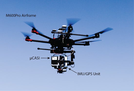
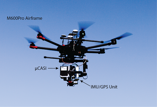
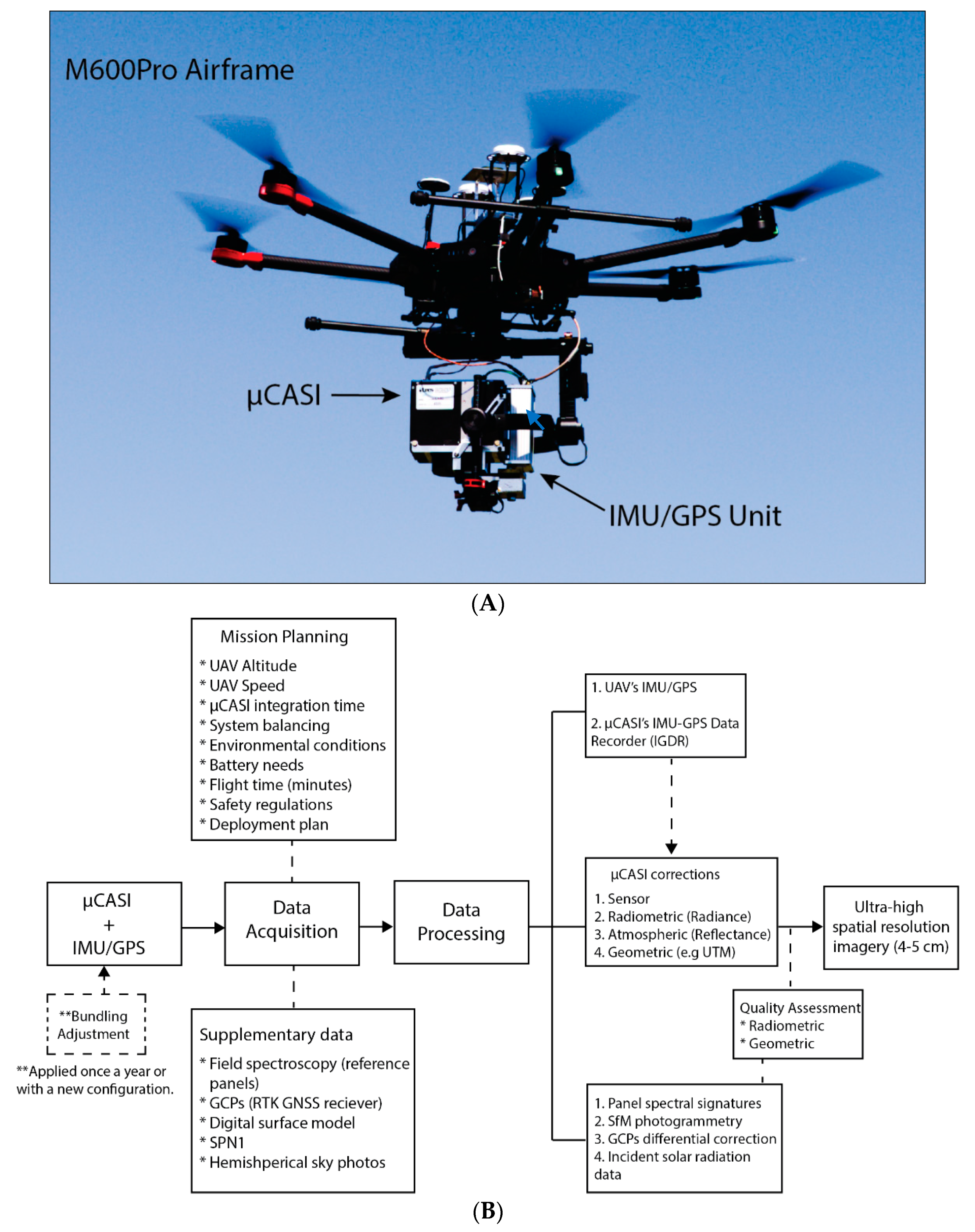
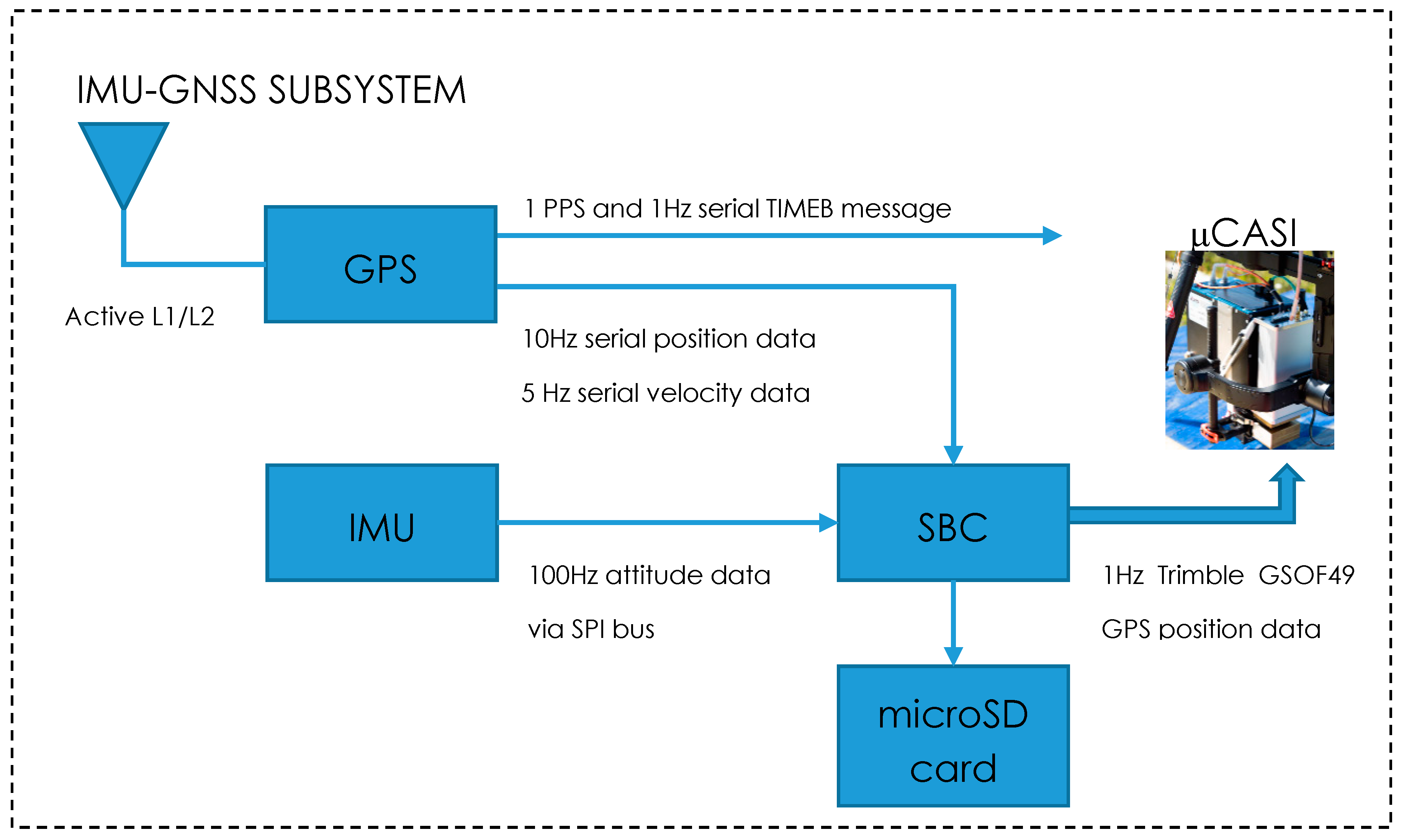
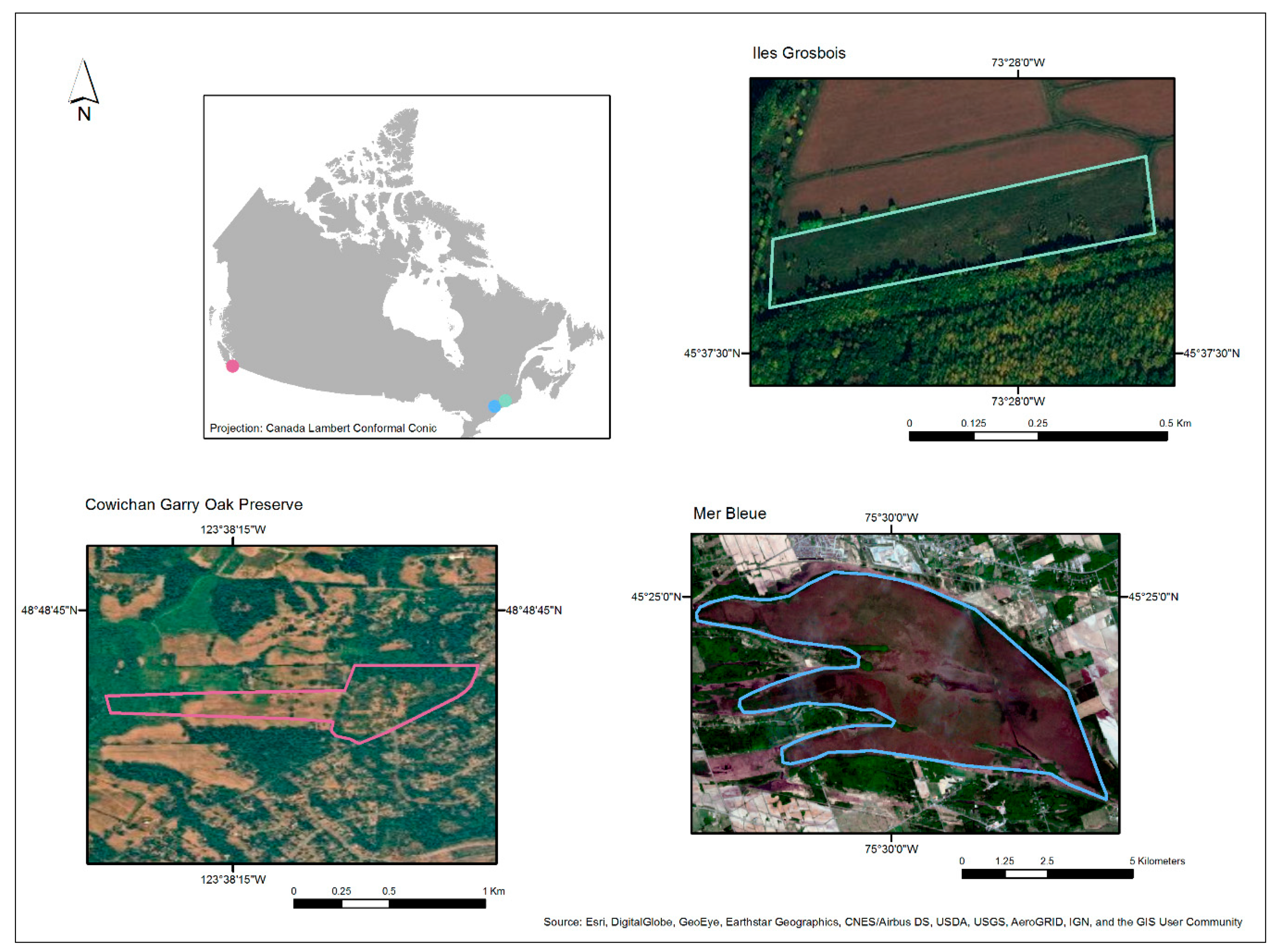
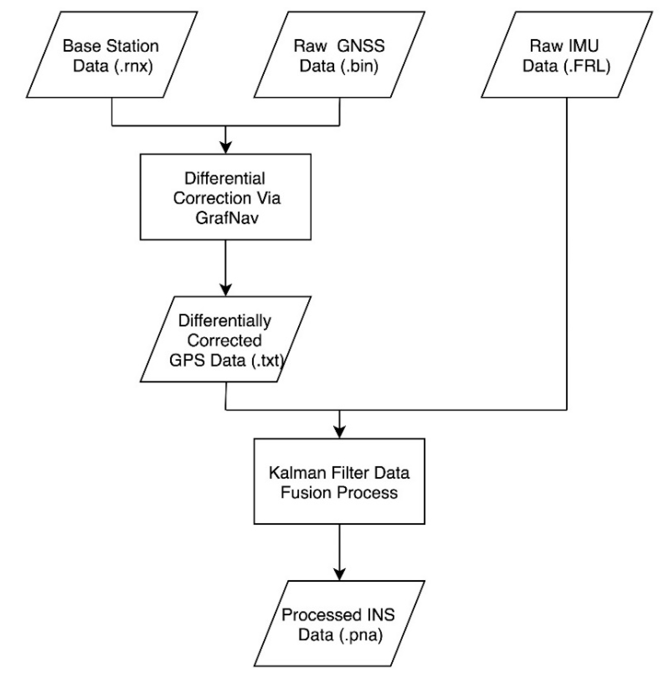
In this paper, we introduce a novel UAV hyperspectral system composed of a heavy lift hexacopter, the Matrice 600 Pro (DJI, Shenzhen, China), the micro Compact Airborne Spectrographic Imager (μCASI; 288 spectral bands from 401–996 nm) (ITRES Research Ltd., Calgary, AB, Canada) and an IMU/GNSS unit developed for the μCASI by the Flight Research Laboratory (FRL) of the National Research Council of Canada (NRC). To the best of our knowledge, this system is the first integration of the μCASI on a low-altitude UAV platform. The μCASI is also usable in an airborne platform (e.g. potential for upscaling comparative studies), providing a new alternative to other commercial systems previously described in the literature. Innovative UAV hyperspectral systems are important to diversify the currently limited availability of options on the market. The UAV-μCASI system is the product of a collaborative effort between the Hyperspectral & Aeromagnetics Group at NRC and the Applied Remote Sensing Laboratory at McGill University. The objective of this system is to complement airborne hyperspectral research for environmental applications as well as to advance the understanding of UAV hyperspectral systems (e.g., geometric and radiometric calibration) as described here. In addition to the description of the UAV-μCASI system, in this work, we present mission planning aspects important for optimizing hyperspectral image quality. We also show results from three case studies addressing peatland research, invasive species monitoring, and endangered tree species mapping as part of the Canadian Airborne Biodiversity Observatory (CABO) project. Our study adds novel aspects related to UAV hyperspectral system implementation and highlights its significant potential for environmental monitoring. The challenges that must be overcome for this type of system to become fully operational (e.g., turnkey) are addressed in the discussion section.

2. Materials and Methods

2.1. UAV-Hyperspectral Imaging System

The UAV-μCASI system is shown in Figure 1A, while Figure 1B shows the different components and processes of the overall system.

Table 1. The weight of the primary components in the UAV hyperspectral imaging system.

Component	Weight (g)
Ronin MX gimbal + battery	2300
μCASI	2760
IMU-GPS Data Recorder (IGDR)	505
Cables	40
Aluminum bracket	280
Counterweight	1090
Differential Real-Time Kinematics (D-RTK) System	820
GPS Antenna and plate	100
Total Weight	7895

illustrates the weight of each component of the payload; for lightweight UAVs, the weight of the payload greatly affects the overall flight time. Significant effort and multiple iterations were dedicated to optimizing the sensor mounting and developing the best configuration to enhance the image quality. Ultimately, our goal was to reduce sensor motion, which in return reduces image distortion and the percentage of rejected pixels (i.e., pixels which cannot be mapped from the original imagery by the geocorrection process). Moreover, the safety of the personnel and equipment during operations were a priority, as per the Transport Canada UAV regulations.

2.1.1. The μCASI Hyperspectral Sensor

The hyperspectral sensor for this work is the µCASI-1920 (SN: 6501) integrated with a Micro-Electro-Mechanical Systems (MEMS) IMU developed at NRC (Section 2.1.3). The µCASI operates in a pushbroom configuration with the line image of 1840 spatial pixels (34.3° Field of View (FOV)) dispersed spectrally via diffraction over 288 spectral (401–996 nm) pixels on a silicon-based Focal Plane Array (FPA). Use of a parallel processed FPA as opposed to a serial processed Charge Couple Device (CCD) detector permits increased frame rates of 100+ frames per second (fps) as opposed to 20 fps for the full detector readout. However, this increase in fps and the associated increase in spatial resolution comes at a cost, as state-of-the-art silicon FPAs are restricted to 30k electron (e-) full well capacity compared to much higher capacities in similarly-sized silicon CCD devices (e.g., 400k e-). The µCASI sensor head measures 16.5 cm long × 10.2 cm wide × 14.5 cm high with a 3.5 cm projection on the bottom containing the fore-optics. Once the desired flight line configuration is programmed, the μCASI operates autonomously in the air using a ‘geofence’ for data recording functions. Image data are recorded at 12-bit radiometric resolution.

2.1.2. Airframe and Hyperspectral Imager Integration

We selected an off-the-shelf airframe, the Matrice 600 Pro (M600P), to implement the μCASI configuration. The M600P is a six-rotor UAV with a maximum takeoff weight of 21 kg (DJI Technical Support, 2017). For navigation, we integrated the DJI Differential Real Time Kinetic (D-RTK) GPS (dual-band, four-frequency receiver) with the A3 Pro flight controller [32]. The A3 Pro flight controller has triple redundant GPS, compass, and IMU units, in addition to advanced software analytics which determines if any of the redundant units have failed. This model also has a greater resistance to magnetic interference than the non-pro version [33], as well as vibration dampeners for the IMUs and the main controller. The μCASI was interfaced to the M600P with the Ronin-MX 3-axis gimbal (±0.02° precision as determined by the manufacturer) which connects directly to the airframe [34], allowing the pilot or flight management software to control the position of the gimbal. Importantly, the Ronin-MX has a ‘car mount’ operational mode designed to prevent the horizon from drifting under the forces sustained from high-speed operations. In the air, this mode keeps the payload steady in challenging conditions and maintains the sensor nadir facing during data collection [35]. The gimbal is further equipped with dampeners to minimize the effect of high-frequency vibration on the payload. The μCASI was mounted to the camera mounting plate of the Ronin-MX via a custom-built aluminum bracket. This same bracket also ensures that the IMU-GPS Data Recorder (IGDR) Inertial Navigation System (INS) (See Section 2.1.3) is rigidly mounted in the same relative position and orientation with respect to the μCASI with less than 1 mm of positional tolerance. This allows for a constant offset and orientation of the two components to be used during successive missions [36]. The combined μCASI-IGDR was manually ‘coarse’ balanced in all three axes (pan, tilt, roll) and subsequently balanced electronically using the DJI Gimbal Assistant software v2.5. The electronic balancing process allows the user to fine-tune the motor stiffness settings and gauge how well the payload is balanced by monitoring the load on each motor separately in real-time. The payload was considered to be balanced when all three motors (pan, tilt, and roll) were using less than 10% total power for maintaining a stable stationary gimbal position. The design of the μCASI with the fore-optics and slit centered on the lower surface of the instrument required the payload to be front heavy in order to provide an unobstructed field of view from the camera mounting plate. Therefore, the use of a counterweight was necessary to balance the tilt axis (Table 1). Both the μCASI (45W of 28V DC power) and the IGDR (4 W) were powered by the M600P from integrated accessory power ports.

2.1.3. The IMU-GPS Data Recorder (IGDR)

The IGDR unit lies within an aluminum housing (16.5 cm × 8.3 cm × 4.4 cm) and contains a tactical grade IMU, a dual-frequency Global Navigation Satellite System (GNSS) receiver, and a Single Board Computer (SBC). The Netburner MOD5441X SBC communicates with the IMU via a serial peripheral interface (SPI) bus and with the GNSS receiver via a serial port. All data received is time-stamped using a 16-bit timer internal to the SBC. A GPS PPS (Pulse Per Second) strobe (time synchronization output) from the GNSS receiver is tied to a hardware interrupt on the SBC and is used to align the SBC’s time to GPS time post-flight. The Analog Devices MEMS-based ADIS16490 IMU is comprised of a triaxial digital gyroscope and accelerometer. It outputs ±100°/sec raw gyroscope data for the pitch, roll, and yaw, as well as ±8 g acceleration data in the x, y, and z directions. During flight, the 32-bit angular rate of rotation and acceleration data is collected at 100Hz, timestamped, and logged to a microSD card onboard the SBC module. Also recorded on the microSD card are position and velocity logs from the Novatel OEM719 GNSS receiver. Raw pseudo-range measurements along with ephemeris data are recorded to a separate file for post-processing Differential GPS (DGPS) corrections. Through a separate serial port, a binary time message is passed along directly from the receiver to the μCASI for time tagging purposes (Figure 2).

The IGDR is also tasked with sending out a Trimble GSOF49 GPS message via Ethernet to the μCASI. This position data is used by the μCASI in real-time to determine its location relative to the user-defined geofence that was loaded preflight. After the flight, the IMU/GPS data files can be retrieved from the SBC’s microSD card using its Ethernet port.

2.2. Sites, Mission Planning, Data Processing, and Testing

2.2.1. Sites

Three sites with distinctive biophysical characteristics and conservation challenges were selected for testing the utility of UAV hyperspectral imagery for ecological monitoring (Figure 3). The first site is the Mer Bleue Peatland Observatory (Ottawa, ON, Canada), which encompasses an ombrotrophic bog with hummock and hollow microtopographic vegetation [37]. Peatlands cover a significant area in Northern regions and play a fundamental role in carbon sequestration [38,39]. Monitoring of peatlands at different spatial scales is important for understanding their response to climate change, and given their generally poor accessibility and fine-scale topographic variation (<50 cm), UAVs have shown potential for mapping these ecosystems [1,40]. Mer Bleue is also located 10 km from FRL, facilitating the implementation of many of the tests at this location. The second site is on Ile Grosbois within the Parc national des îles-de-Boucherville (adjacent to Montreal, Quebec), where native vegetation is currently threatened by the common reed Phragmites australis ssp. Australis. Assessing the spectral differences between the native grasses, herbaceous plants, and the common reed is important for understanding how the invasive species spread through time, and therefore, it is useful for defining the appropriate control and/or eradication practices. The third site, located in Duncan, British Columbia, is the Cowichan Garry Oak Preserve (CGOP). Garry Oak (Quercus garryana) ranges from British Columbia to California. It is a threatened ecosystem in Canada due to fragmentation and invasive species affecting the native wildflowers and grasses [41]. Our goal at the CGOP was to acquire imagery to capture the variation in forest structure (open areas to high tree density), characteristic of this ecosystem.

2.2.2. Mission Planning

Flight lines were preplanned with ArcGIS 10.6 (ESRI, Redlands, CA, USA) to precisely determine the heading and the actual flight path, as well as the location of the hover points at the start of each flight line within the μCASI’s user-defined geofence (Figure 4). At each hover point, the UAV comes to a standstill for twenty seconds while the μCASI acquires the dark current and spectral lamp scan lines required for optimal image processing. Sufficient space is provided between the hover point and the beginning of the effective image area (Figure 4) to ensure the gimbal and airframe have re-stabilized following acceleration. An overlap of 30% considering a maximum roll less than 5° was planned for adjacent flight lines. The flight plans were uploaded to DJI Ground Station Pro (GSP) as waypoint missions. GSP also served as the auto-pilot for the A3 Pro flight control system. Considering the near maximal takeoff weight of the aircraft, flight time and flight distance were limited to approximately 10–12 min (~1200 m) including the transit to and from the start and end points. Transit speeds are greater (e.g., 10 m/s) than the effective imaging speed (e.g., 2.7 m/s). This limit further allowed us to conserve approximately 30% battery power in case of an emergency or stronger than anticipated wind during flight. While GSP initiated the takeoff and the waypoint flights, landings were carried out manually by the pilot for the safety of the personnel and equipment. Portable wood or PVC platforms were used to minimize dust in the slit of the μCASI and to provide a solid and level landing surface. The encrypted flight logs (GPS position and attitude) from the M600P were extracted with DatCon 3.6.1 for further analysis.

Because the composition of the landscape in the three ecosystems tested here was primarily composed of vegetation with a low response in the blue wavelengths, the sensitivity of the µCASI was enhanced by optimizing the integration time for materials with low reflectance in these wavelengths (e.g., 9–10 ms). Had the scenes been comprised of a material such as concrete with naturally higher reflectance in the blue wavelengths, the signal would have saturated; this was not a concern for vegetated targets.

2.2.3. Flight Speed Tests

To establish the optimal flight speed for data acquisition, six flight lines were flown over the Mer Bleue Peatland site at an altitude of 30 m AGL. The UAV was flown at speeds of 1.8, 2.7, 5.4, 8.2, 10.9, and 13.6 m/s for each flight line, respectively. The processed IGDR data (Section 2.2.4) was used to determine the optimal speed for hyperspectral data acquisition. In particular, the optimal speed was established by identifying the flight line that minimized the roll and pitch for the effective image area, not taking into account the pre and post-flight acceleration and deceleration regions (Figure 4). The spatial density of the GPS observations from the IGDR’s GNSS receiver was further taken into consideration when determining an optimal flight speed as well as the resulting pixel aspect ratios and along-track coverages.

2.2.4. IGDR Data Processing

Receiver Independent Exchange Format (RINEX) GNSS observation files were retrieved from the Smartnet North America (Smartnet, Atlanta, GA, USA) active control station(s) closest to the study sites (<50 km). Additionally, precise GNSS orbit and clock ephemerides were downloaded from the Natural Resources Canada’s Canadian Geodetic Survey. These data were used as the base station data for the differential correction of the GNSS data from the IGDR in GrafNav (Novatel, Calgary, AB, Canada). The GNSS data (down-sampled from 10 Hz to 1 Hz) was combined with the raw IMU data in a Kalman filter process developed in-house, outputting a 100 Hz dataset consisting of the latitude (°), longitude (°), altitude (m), pitch (°), roll (°), heading (°), North velocity (m/s), East velocity (m/s), and downwards velocity (m/s) (Figure 5). This combined dataset was then used in the geocorrection process.

2.2.5. Bundling Adjustment

During the geocorrection process, the position and attitude of the μCASI sensor are characterized by the IGDR (Section 2.1.3). However, its reference point does not coincide with the optical center of the mounted μCASI, which is a common issue in these systems [36]. The bundling adjustment process was carried out to characterize and account for this spatial offset. In this process, 10 bundling flight lines (6 in the East/West orientation, 4 in the North/South orientation) were collected over the Mer Bleue site that contained 45 ground control points (GCP). The geographic location of each GCP was determined with a separate GNSS receiver (Section 2.3.1). The flight plan was designed with 80% overlap between adjacent flight lines. Each GCP was identified in the imagery and a fixed spatial offset between the IGDR reference point and the μCASI was calculated based on the position of each GCP, as viewed from multiple images. The geographical error of the GCPs was used to determine the significance of the bundling adjustment.

2.2.6. Radiometric, Atmospheric and Geometric Correction of the μCASI Imagery

The hyperspectral data underwent a series of preprocessing steps using software modules developed by the instrument manufacturer and commercial software. The first step corrected the μCASI laboratory calibration for shifts in the spatial-spectral sensor alignment [16] that are believed to be caused by changes in temperature and pressure. The second step estimated and removed offset contributions (i.e., electronic offset, dark current, frame shift smear, internal scattered light, and 2nd order scattered light). The resulting offset-corrected pixel signal was then converted into units of spectral radiance (μW·cm⁻²·sr⁻¹·nm⁻¹). In the third preprocessing step, the laboratory-measured spectral smile was removed by resampling the spectral data across the field of view of the sensor to a common wavelength array. Next, the images were atmospherically corrected with ATCOR^®4 (ReSe Applications GmbH, Wil, Switzerland). Subsequently, the processed attitude and position data from the IGDR (Figure 5) was time synchronized with the hyperspectral data. In the final preprocessing step, the hyperspectral images were geocorrected using the IGDR’s GNSS position and attitude to construct the sensor orientation for each scanline in the imagery. Afterward, the data from each pixel was projected into a physical space defined by the horizontal and vertical datum. While projecting the data and calculating the precise location of each pixel in the image that is not geocorrected, a digital surface model (DSM) (Section 2.4.2) was used as an initial input to account for the terrain of the imaged environment. A nearest neighbor interpolation method was applied to sample the projected data at the desired spatial resolution. In order to carry out quality control assessments of the imagery, the radiance images were also geocorrected.

2.3. Geometric and Radiometric Assessments

2.3.1. Geometric Assessment

Circular orange plastic disks (30 cm and 15 cm in diameter) with a contrasting white and black “X” across the center were placed throughout the plots as the GCP targets for the geometric assessment of the μCASI imagery and as GCPs for the Structure from Motion-Multiview Stereo (SfM-MVS) workflow (Section 2.4.2). The positions of the disks in the x, y and z axes were measured with an Emlid Reach-RS RTK GNSS receiver (St Petersburg, Russia). RTK correction was provided by the Smartnet North America NTRIP (Networked Transport of Radio Technical Commission for Maritime Services (RTCM) via Internet Protocol) casting service on an RTCM3-iMAX (individualized Master-Auxiliary) mount point utilizing both GPS and GLONASS constellations. iMAX generates corrections for a real reference station and the baselines between the base station and the measured points can, therefore, be directly re-measured, thus resulting in GCP positions that are both traceable and repeatable. An image from Mer Bleue (30 m AGL, 2.7 m/s) was used to test the benefit of incorporating a DSM into the geocorrection process to mitigate parallax errors (Section 2.4.2). The positional accuracy of the geocorrected image was determined in relation to the GCPs identified in the image.

2.3.2. Radiometric Assessment

An ASD FieldSpec 3 (Analytical Spectral Devices, Boulder, CO, USA) spectroradiometer with a 2 m fiber extension was used to collect reference spectra of four calibration targets placed in at least one flight line per plot. The four targets consisted of 2% and 50% Spectralon™ panels (10”), an 18% Flexispec™ (50 cm) sheet, and a 10% Permaflect™ (50 cm) panel (Labsphere, North Sutton, NH) (Figure 6). A 10” 99% reflective Spectralon™ panel was used as the reference for all measurements. Measurements were carried out via the panel substitution method to account for a first-order correction of the 8°:hemispherical reflectance factors provided with a new reference panel to the 0°:45° biconical reflectance viewing and illumination geometry factors of Spectralon™ according to the methodology described in Reference [1]. These measurements of panel reflectance were used to assess the quality of the atmospheric correction of the μCASI imagery.

2.4. Supplementary Data

2.4.1. Incident Solar Radiation and Sky Condition Measurements

Upon reaching each field site, the first instruments set up to collect data were the SPN1 Sunshine Pyranometer (Delta-T Devices, Cambridge, UK) and a Canon EOS60D camera with an ultra-wide-angle lens (Sigma 4.5 mm F2.8 Ex DC Hyper Sonic Motor Circular Fisheye lens) on an intervalometer (10 min) (Figure 7A,B). The pyranometer and camera collect data throughout the entire day’s deployment in order to characterize the changing illumination conditions. The photographs provide an important visual record of the atmospheric conditions and can be referenced to help understand the findings in the other datasets. The pyranometer measures incident solar radiation (both diffuse and global) with seven thermopile sensors and a computer-generated shading pattern. It is connected to a small field laptop that logs the measurements at set intervals (e.g., 10 sec). Figure 7B shows an example of incident solar radiation (indirect, diffuse, and total) for the CGOP site from 25 July 2018.

2.4.2. Digital Elevation Model Generation

In order to improve the overall geocorrection of the μCASI data (Section 2.2.5), near coincidental aerial photographs were collected for 3D surface reconstruction through a SfM-MVS workflow [24]. A DJI Inspire 2 (3.4 kg 4-rotor) UAV was used with an X5S camera. This camera has a micro 4/3 sensor (rolling shutter), an integrated 3-axis ±0.01° gimbal, and a DJI MFT 15 mm/f1.7 aspherical lens (72° diagonal field of view). The photographs from the X5S each have an image size of 5280 × 3956 pixels. All photographs included the geolocation of the center of the frame and the altitude in the EXIF (Exchangeable image file format) data. SfM-MVS products consisting of an orthomosaic, dense 3D point cloud, and digital surface model (DSM) were generated with Pix4D Mapper Pro [24,27,28,42].

3. Results

Our UAV-μCASI system’s payload weighs a total of 7895 g (Table 1). Allowing for a remaining 30% battery charge at landing as a safety measure resulted in flight times of 10–12 min in low wind conditions with high-performance 5700 mAh batteries. At a flight speed of 2.7 m/s it is possible to acquire a flight line of up to approximately 1200 m. At an altitude of 45 m AGL the image swath is 27 m wide with a 4 cm geocorrected pixel size.

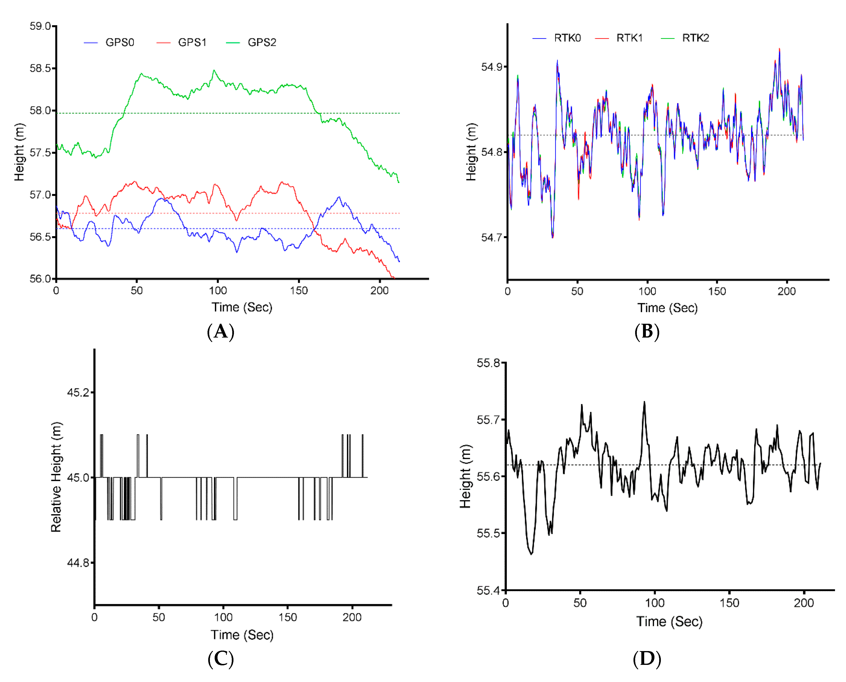
Figure 8 shows an example of the uncorrected GPS (Figure 8A) and RTK (Figure 8B) logs for a flight line from Ile Grosbois. Values in Figure 8A,B,D represent orthometric height, whereas 8C illustrates relative height (AGL) as recorded by the M600P’s barometer. Differences in height recorded by the three GPS receivers are 0.18 m between GPS0 (μ = 56.60 m) and GPS1 (μ = 56.78 m), and 1.37 m and 1.19 m compared to GPS2 (μ = 57.97 m), respectively. The RTK corrected data in Figure 8B reveals no difference in the mean orthometric height (μ = 54.82 m) between the three receivers. Height measurements above ground provided by the barometer (Figure 8C) indicate a maximum difference of 10 cm variation during flight, while the IGDR (Figure 8D) recorded an average orthometric height of 55.62 m (range 0.27 m).

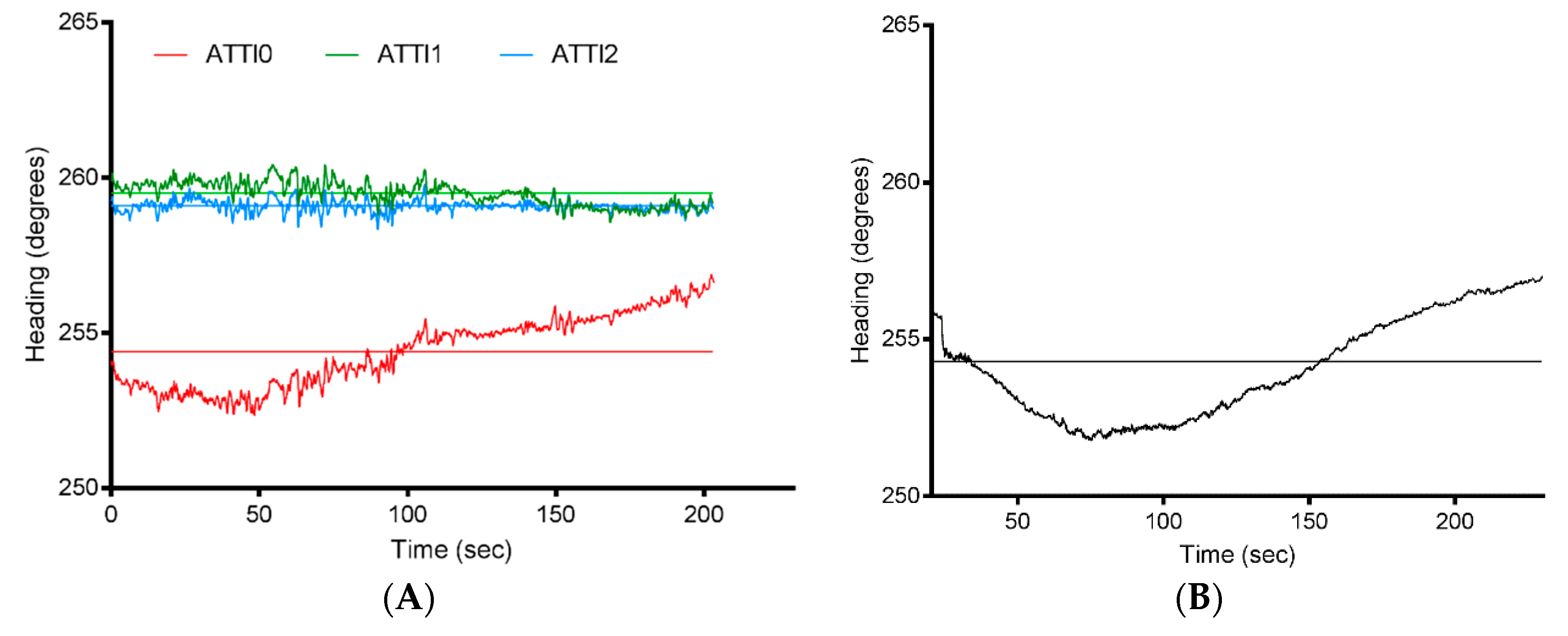
The heading recorded by the A3 Pro’s IMUs from the same flight indicates a larger variation between ATTI0 (mean 254.4°) to ATTI1 (mean 259.5°) and ATTI2 (mean 259.1°). ATTI0 recorded a similar mean heading to that of the IGDR (mean 254.3°) (Figure 9).

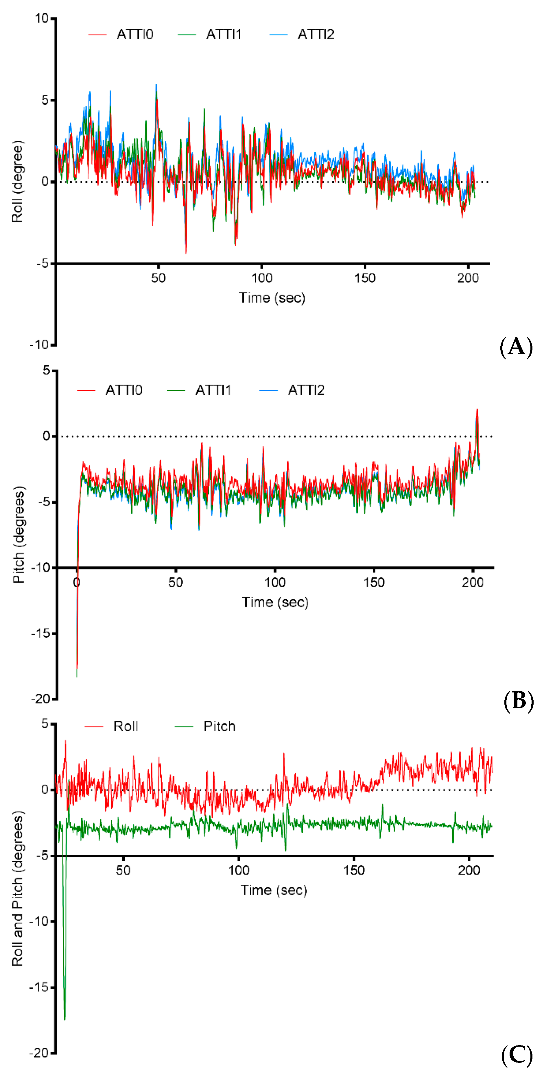
Attitude data for the M600P from the same Ile Grosbois flight line illustrate congruent measurements with minimal differences in roll (Figure 10A) and pitch (Figure 10B) from the three IMUs. The magnitude of the roll recorded for the airframe is larger than for the payload (Figure 10C) due to the stabilization provided by the gimbal. Corrections by the airframe in response to wind gusts can be seen in Figure 10A between 50 and 90 seconds into the flight. The large negative pitch at the beginning of the flight line is characteristic to the manner in which rotorcraft UAVs transition from a stationary position to forward motion; the nose of the airframe initially pitches down and then levels off as the flight speed is attained. The reverse can be seen when the airframe slows down to a stationary position at the end of the flight line. It is important to note that the airframe maintains a slight forward pitch during flight (~3.5°–4°). From the IGDR the large negative pitch recorded as the airframe begins to pick up speed lasts less than 2 seconds before the gimbal compensates for the motion. As expected, due to the stabilization provided by the gimbal during the flight, the average roll (0.4° ± 1.1°) and pitch (−2.7° ± 0.5°) recorded by the IGDR are less than that of the airframe (roll μ = 0.74° ± 1.2°; pitch μ = −3.9° ± 0.96°). It is important to note the maximum value of pitch recorded during flight (outside of the acceleration and deceleration regions) is −7.0° for the airframe and −4.7° for the gimbal.

Our speed test results from the Mer Bleue site indicate that the optimal flight speed to maximize the μCASI image quality is approximately 2.7 m/s (Figure 11,

Table 2. The along and across-track spatial coverage per pixel at different flight speeds for the μCASI given an altitude of 30 m AGL. XTR—across-track resolution; ATR—along-track resolution.

Flight Speed	Across Track FOV (cm)	Along Track Resolution (FWHM cm)	Along Track Coverage (FHWM %)	Pixel Aspect Ratio (XTR/ATR)
1.8 m/s	1.0	2.1	107.2	0.47
2.7 m/s	1.0	2.9	98.8	0.34
5.4 m/s	1.0	5.4	90.3	0.19
8.2 m/s	1.0	7.9	87.4	0.13
10.9 m/s	1.0	10.3	86.0	0.10
13.6 m/s	1.0	12.7	85.2	0.08

). Pitch and roll recorded by the IGDR at speeds of 8.2–10.9 m/s revealed a proportional increase in the distance traveled in the air to the gimbal beginning to compensate, resulting in longer lead-in distances before quality imagery could be acquired. At 13.6 m/s the gimbal remained at a pitch in excess of −20°, while at 10.9 m/s the pitch ranged from −8° to −7° during the majority of the flight. For the 1.8 to 5.4 m/s speeds the roll and pitch were in the same range as seen in Figure 10C. Flight speed further affected the number of GNSS observations in each flight line (Figure 11). As expected, at lower speeds, less interpolation with the Kalman filter between actual observations of the spatial position of the μCASI is necessary; with a constant frequency of the GNSS observations following differential correction, faster speeds result in larger spatial gaps. At the 5.4–13.6 m/s speeds, the distance required for the M600P to achieve full speed followed by deceleration at the end of the flight line can be seen in the variable distances between observations.

Flight speed also affected the along-track resolution, coverage, and overall pixel aspect ratio (Table 2). As the speed increases, given a constant altitude, integration time and frame time, the pixel aspect ratio (ATR/XTR) increases. At 13.6 m/s for example, each pixel is nearly 13 times longer than it is wide. The along-track coverage expressed as the percent covered at the Full-Width-Half-Maximum (FHWM) of the point spread function in the along-track direction decreases with increased speed. At faster flight speeds, more pixels would need to be summed in the across-track direction, increasing the overall geocorrected pixel size. At 2.7 m/s we maximize the along-track coverage (98.8%) without oversampling. Also, minimal summation is required in the across-track direction for 3–4 cm geocorrected pixels.

Based on the bundling adjustment process carried out at the Mer Bleue site, our results indicate a decrease of 40.9 cm in the magnitude of the spatial position error compared to the location of the GCPs without the bundling adjustment applied in the geocorrected image (4 cm pixel size) (

Table 3. A comparison of the effect of the bundling adjustment in the geocorrection process at Mer Bleue: Ground control point (GCP) location vs. geocorrected imagery.

	No Bundling Adjustment		Bundling Adjustment
Variable	Easting	Northing	Easting	Northing
Mean (m)	0.348	−0.484	0.186	−0.012
Min (m)	−0.016	−0.771	−0.078	−0.191
Max (m)	0.867	−0.029	0.587	0.251
Standard deviation (m)	0.298	0.237	0.185	0.129
Magnitude of Error (m) *	0.596		0.187
Direction (°TN)	144.27		93.63

* Magnitude of the error represents the error vector calculated as: √(Δ__E² + Δ__N²).

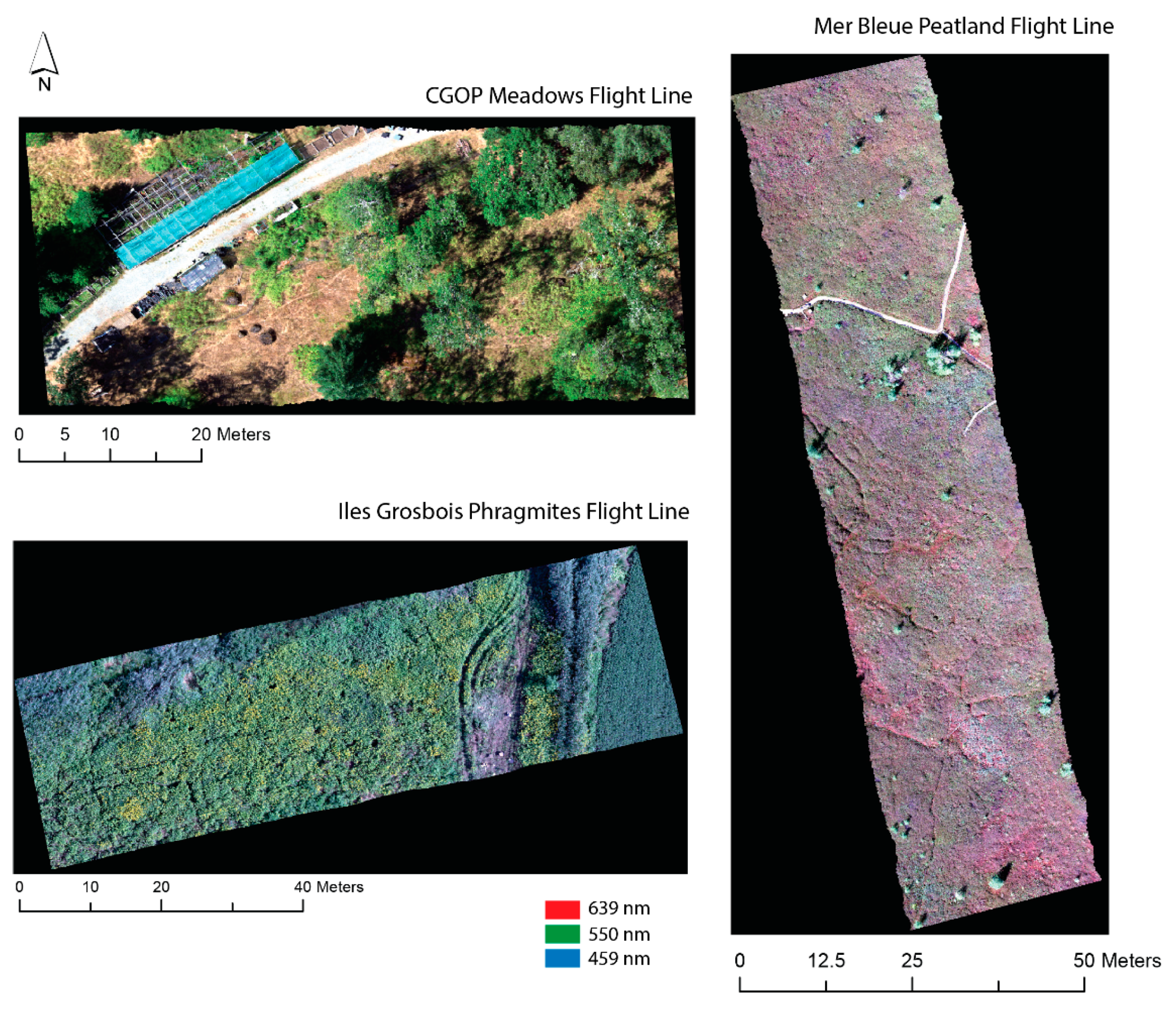
). The spread around the mean also decreases from 0.298–0.185 cm in the Easting direction (Δ_E = 11.3 cm), and from 0.237–0.129 cm (Δ_N = 10.8 cm) in the Northing direction (Table 3). Figure 12 illustrates an example of the geocorrected images in radiance (μW/cm² sr nm) for the three study areas derived using the bundling adjustment process.

Table 4. Per-pixel image results and data acquisition summary for ultra-high resolution geocorrected hyperspectral images for study sites derived from UAV-μCASI system. XTR—across-track resolution; ATS—along-track pixel spacing; ATR—along-track resolution.

Location	No. Image Pixels	% Pixels Rejected	No. Rejected Pixels	Altitude AGL(m)	XTR (cm)	ATS (cm)	ATR (cm)	Geocorrected Res. (cm)
Mer Bleue	2,266,680	0.10	2363	45	1.52	2.43	3.19	4.0
Ile Grosbois	1,547,233	0.17	2711	45	1.47	2.43	3.16	4.0
CGOP	844,554	0.79	6681	60	1.96	2.43	3.41	5.0

indicates that for all lines shown in Figure 12, the percentage of rejected pixels following geocorrection ranges from 0.1% at Mer Bleue to 0.79% at CGOP. The use of a DSM in the geocorrection process at Mer Bleue (

Table 5. Results on the effect of using a DSM in the geocorrection process at Mer Bleue.

	No DSM		With DSM
	Easting	Northing	Easting	Northing
Mean	−0.437	−0.019	−0.410	−0.016
Min	−0.763	−0.202	−0.763	−0.162
Max	−0.053	0.256	−0.093	0.256
STD	0.158	0.105	0.151	0.096
Magnitude of Error *	0.437		0.410
Direction (°TN)	267.48		267.80

* Magnitude of the error represents the error vector calculated as √(Δ__E² + Δ__N²).

) resulted in small differences between the Easting and Northing coordinates between the GCP locations with and without the DSM (Δ_E = 2.7 cm, Δ_N = 0.3 cm). The magnitude of the error for the difference is 2.7 cm.

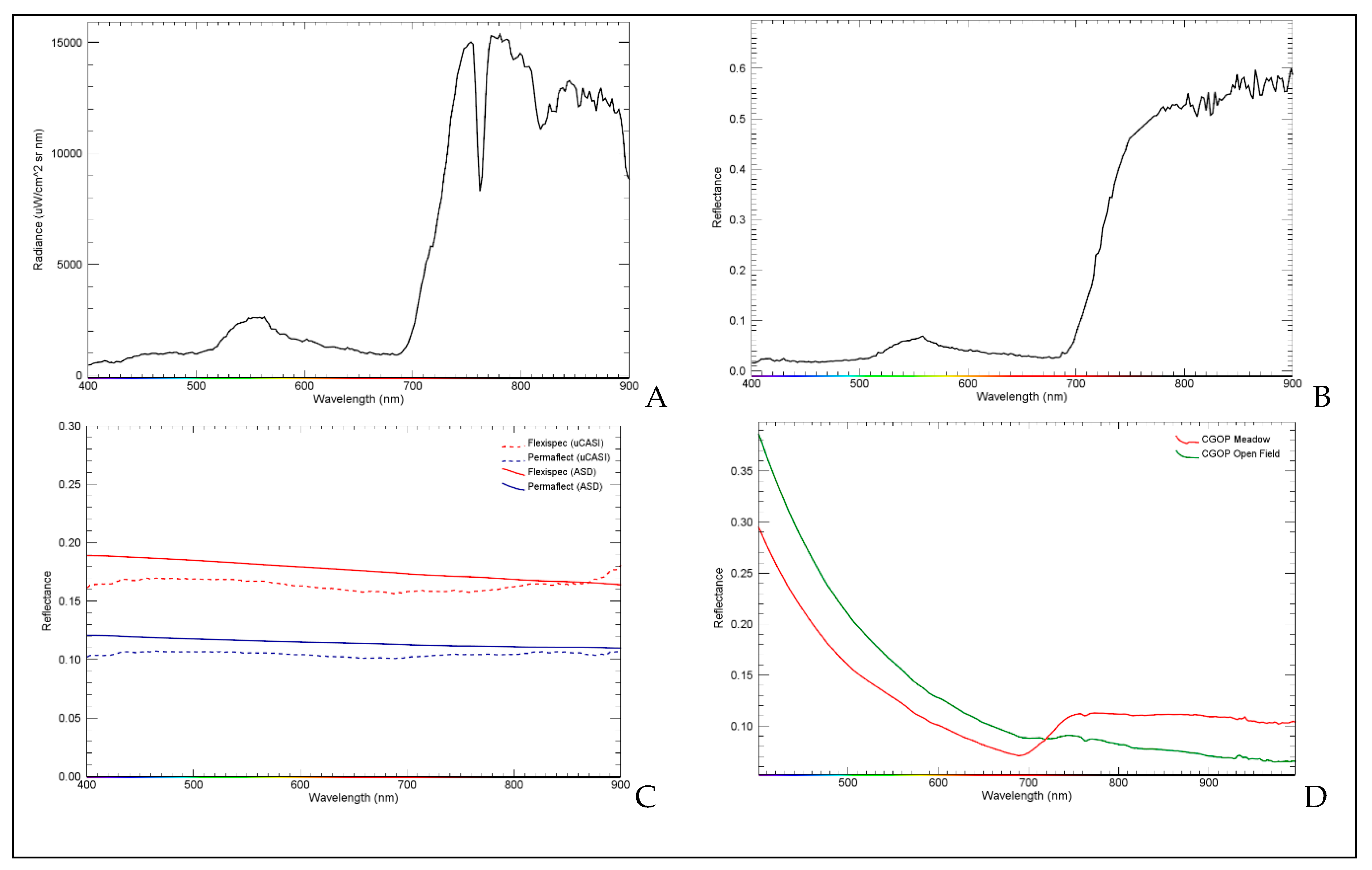
An example of the spectral profile of a Garry Oak canopy pixel is shown in both radiance (Figure 13A) and reflectance following atmospheric correction with ATCOR^® 4 (Figure 13B). Figure 13C illustrates the similarities between the ASD in-situ field spectral (Section 2.3.2) measurements of the Flexispec™ and Permaflect™ panels and corresponding pixels from the atmospherically corrected μCASI image. Across the 400–900 nm wavelength range, for the 18% Flexispec™ panel, the absolute difference is 1.5 ± 0.8% between the ASD and μCASI. For the 10% Permaflect™ panel, the absolute difference is 1.0 ± 0.5%. Due to this high degree of similarity between the in-situ measurements and the imagery, the scene-based calibration from ATCOR^® 4 was not applied because it would have introduced additional uncertainties rather than refinements of the atmospheric correction.

As seen in Figure 13D, due to the proximity of the trees to the location of the panels, in-scattering can be seen in the diffuse illumination measurement of the 99% Spectralon™ panel. This contamination is not seen in the measurement from the open field. As seen in Figure 14, panels in the CGOP Meadow flight line were placed in the largest open area. Nevertheless, due to the height of the trees on either side, in-scattering was unavoidable. Under these circumstances, the panels were used solely for verification of the quality of the atmospheric correction.

4. Discussion

Our study brings to the attention of the remote sensing community a new micro hyperspectral sensor, the μCASI, which had not been previously discussed in the literature (e.g., [43]). One of the most notable advances made by our study is the demonstration of the radiometric and geometric data quality of the UAV-μCASI system. For example, the agreement between the in-situ field spectral measurements of the laboratory calibrated reference panels and the atmospherically corrected imagery suggests the imagery from our system can be used with a high degree of confidence for research questions requiring spectral fidelity. Our study further provides insights into aspects of data collection that influence the quality of the imagery and showcases the importance of the collection and rigorous processing of supplementary in-situ data (e.g., SPN1, field spectra, GCPs) for generating and assessing the quality of the imagery. Because of the ultra-high spatial resolution of the geocorrected imagery, another fundamental contribution of our study is the detailed investigation of the performance of the airframe, gimbal, navigation system, and the IGDR. These aspects, while often overlooked, provide valuable insights into optimizing flight planning for a given system or configuration, as discussed below.

We demonstrate that there are a few fundamental aspects to consider when implementing a UAV based pushbroom hyperspectral system, given the high spectral resolution (e.g., >200 bands) and ultra-high spatial resolution (<5 cm) at which the imagery is acquired. Ultimately, these high-end and expensive systems (~US $100,000–350,000) have shown great potential for mapping and ecosystem characterization in different applications [26,29,44]. However, they are not 100% ‘out-of-the-box’ operational yet (i.e., “turnkey”), still requiring considerable effort from expert users. Including ancillary data collection equipment (e.g., the RTK GNSS receivers, pyranometer, and field spectrometer), our system is still within the range of other expensive hyperspectral systems and requires a crew of 5–7 people for full deployment. Further research is needed to fully understand the integration of the different components and aspects to decrease system costs. For instance, our research group initially debated whether the hyperspectral sensor should be hard mounted (e.g., [26]) or mounted on a gimbal (e.g., [29]). The GNSS positioning and attitude information from the airframe’s IMU(s) are important (but not available for all UAV platforms) to assess the potential errors introduced by the inaccuracies of each component. Moreover, the UAV’s flight logs provide data on the precision of the flight lines and whether there are notable changes to planned flight paths caused by external forces (e.g., wind) or system failure. These logs are also used for identifying geolocation errors to within a few centimeters of accuracy [45], and with the right configuration, they could be used for direct georeferencing when no GCPs are available [46]. For instance, our results indicated important differences between the three GNSS receivers of the A3 Pro flight controller and the integrated RTK corrected altitudes (Figure 8A,B). As expected, variations in the GNSS receivers are minimized by the RTK enabled flight controller. Height variations from the corrected position data are very similar to those of the μCASI’s IGDR (Figure 8B,D). A direct comparison between the absolute values can only be done after standardization of the horizontal and vertical coordinate systems. For example, the IGDR records the 3D position information in latitude/longitude WGS84 (horizontal datum), and EGM96 for the geoid, whereas the A3 Pro uses the same horizontal reference frame, but at the time of data collection it calculated the orthometric height based on the EGM2008 geoid. A further complication is that the base station data from Smartnet is provided in NAD83CSRS for the horizontal reference frame (with the CGVD2013 geoid). Furthermore, the requirements of the geocorrection module are input data in WGS84 with EGM96 providing an output in UTM (WGS84). As such, care must be taken with all spatial coordinates to ensure no error is introduced through reprojection.

Heading data obtained from the UAV platform and the μCASI’s IGDR showed better congruence with the primary IMU (ATTI0) (mean difference 0.3°) than the redundant systems (ATTI1, ATTI2) (Figure 9A,B). Furthermore, extracting the attitude logs from the platform allowed us to assess the utility of the gimbal. Roll and pitch results revealed that once the system is stable (i.e., flight speed has been achieved), lower roll and pitch are recorded by the IGDR than from the M600P airframe, as expected. In order to travel in a forward motion, a greater force from the rotors in the back cause the nose to tilt down; at a speed of 2.7 m/s, the M600P maintained a forward pitch of 3.5–4°. Commercial off-the-shelf systems such as the M600P are subject to ongoing mandatory firmware and software updates by the manufacturer. These updates may include “minor” changes that could have profound impacts on the data quality when the airframe is used for the hyperspectral image collection. For example, the geoid used by the M600P at the time of data acquisition may change in a future update (DJI Technical Support, personal communication, 2018).

A thorough technical understanding of the hyperspectral sensor and mission planning are also essential for collecting geometrically and radiometrically accurate data. For example, because the μCASI is a pushbroom sensor, the speed and integration and frame times play a role in determining the pixel size. At a given altitude, integration, and frame time, faster speeds result in longer pixels in the along-track (forward) direction than in the across-track direction (Table 2). Moreover, flight speed also affects the number of GNSS positions recorded by the IGDR (Figure 11) that are necessary for image post-processing. Our ideal speed of 2.7 m/s is comparable to that used by Reference [29] in two study areas in France (i.e., 3 m/s and 4 m/s), and by Reference [26] (i.e., 2.5 m/s) using a different hyperspectral pushbroom sensor. Also, given the configuration of the UAV-μCASI system, to account for the boresight offset (i.e., offset between INS and sensor) [29,36], the bundling adjustment results (Table 3) showed an improvement of approximately 2–3 geocorrected image pixels in the Easting and Northing directions (Δ_E = 11.3 cm; Δ_N = 10.8 cm). Mission planning also depends on the sensor characteristics. For example, we currently hover the system within the geofence at the beginning of each line in order for the μCASI to complete its internal calibration. The UAV must then exit the geofence at the end of each flight line in order to complete writing the file to the disk.

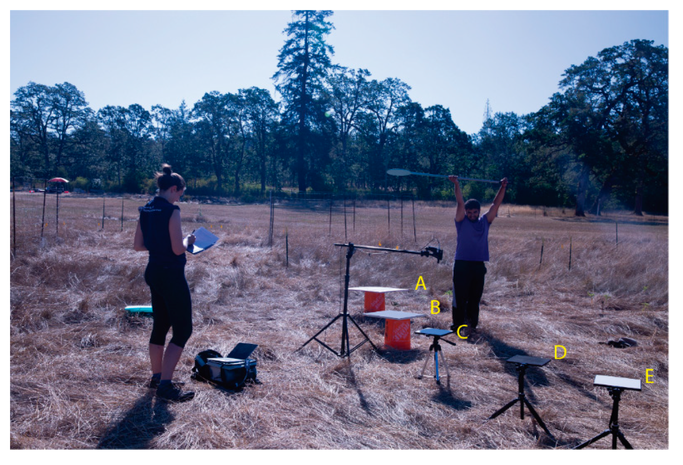
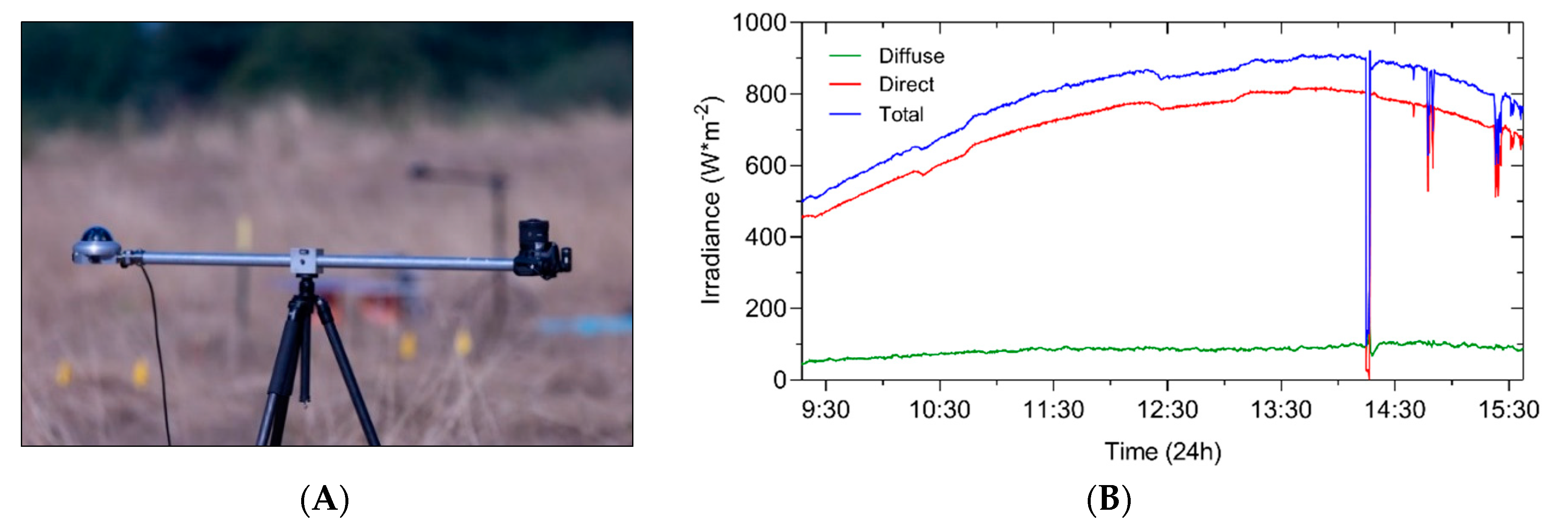
Because mission planning takes into account wind speed, solar illumination, ambient temperature, topography and current UAV regulations in Canada, deployments with the UAV-μCASI are still an intricate task. Wind (sustained wind speed and gusts) is a primary factor that affects the system stability and quality of the data. We limit data collection to sustained wind speeds below 9.7 knots (5 m/s) with maximum wind gusts less than 19.4 knots (10 m/s). Not only is this important for the actual system, but also in high wind conditions the movement of the vegetation increases, resulting in increased motion blur and an overall decrease in image quality both for the μCASI and the SFM-MVS data. The requirement for clear sunny days with only minimal homogeneous cloud cover affects the number of days that the system can be deployed. Because in many instances we deploy in areas with variable sky conditions, the use of ultra-wide-angle photographs and the pyranometer for incident solar radiation improves our understanding of the radiance products (Figure 7A,B). To date, we have operated the UAV-μCASI in air temperatures from 10 °C at Mer Bleue in the spring to 34 °C at CGOP in the summer, where a cooling system was necessary for the batteries before recharging them.

Topography is a variable that can greatly affect the geocorrected imagery, and therefore, implementing a DSM is recommended [35]. We consider vegetation to be a considerable component of the topography. For example, at CGOP, neighboring pixels on the border of a tree crown could have 20 m vertical separation between them (i.e., tree crown vs. ground) which leads to changes in viewing geometry. For pixels <5 cm, parallax errors induced by this difference require additional research. Currently, the geocorrection module cannot correct for such large parallax errors with the very small pixels, but improvements to the module are currently under development and will be tested in the future. While we are continuing to improve the geocorrected output for the three sites, the number of rejected pixels is minimal (Table 4) and the spatial errors are within 2–3 pixels. As an initial assessment, the comparison between the atmospherically corrected μCASI pixels and the ASD in-situ field spectra indicate minimal differences (Figure 13). Additional improvements are necessary to remove the residual atmospheric features in the NIR wavelengths. The spot size for the ASD in-situ field spectral measurements is 13.9 cm diameter. With the along-track resolution of 3.24 cm (XTR = 1.62 cm, ATS = 2.43 cm) for this flight line and taking into consideration the theoretical point spread function of the μCASI, the area contributing to the signal from both instruments is similar. Further work also needs to consider characterizing and minimizing BRDF effects. Finally, regulations play a significant role, and they evolve rapidly. Airspace and proximity to aerodromes, for instance, are factors affecting the maximum altitude at which the data can be recorded.

Most airborne hyperspectral image acquisition systems and associated processing theory and methods have been developed over the last two decades for larger pixels obtained from aircraft platforms (e.g., 1–5 m) [1,4]. In these cases, positional errors of tens of centimeters (or even several meters) were considered excellent because they were subpixel. With the ultra-high spatial resolution obtained from UAV platforms, these relatively ‘small’ errors become increasingly important. An error of 10 cm is no longer subpixel; it is on the order of 3–4 pixels. Furthermore, the parallax errors that were readily dealt with for most vegetated terrain (even forest) from an aircraft acquiring imagery from 1000–3000 ft. and above are magnified in the low altitude UAV flights with ultra-fine pixels, resulting in complications analogous to extremely mountainous terrain. These new challenges will require development or refinement of algorithms specifically targeted to low altitude UAV based hyperspectral imagery, as well as more precise hardware such as the GNSS systems specifically designed with the ultra-high spatial resolution data in mind. For increasing the operational environment of the UAV-based hyperspectral data, advances are needed in battery power for longer flight times. However, this is a trade-off because illumination conditions and the ability of the system to record and store the data onboard must also be considered. An extremely long flight time (e.g., several hours) is not necessarily useful if the window of appropriate illumination conditions for acquiring the data is narrow, or the system cannot store such a large volume of data onboard. A single 600 m long geocorrected flight line (4 cm geocorrected pixel size) from the UAV-μCASI system is >50 GB (raw file size ~22 GB). Computational resources for not only writing the file to the disk upon acquisition (i.e., I/O throughput, storage media write speed) but also for preprocessing, analysis, and long term storage need to be kept in mind when planning UAV hyperspectral data acquisition campaigns.

5. Conclusions

Our hyperspectral system in combination with a custom-built INS with associated processing routines resulted in geocorrected lines with minimal distortion and rejected pixels for three sites with different structural and ecological characteristics: an abandoned agricultural herbaceous field, a Garry Oak forest, and a peatland. The comparison with GCPs indicates positional errors of a few centimeters (Table 3 and Table 5). Given the ultra-high spatial resolution, high geo-positional accuracy is needed for ecosystem characterization. The minimal differences between the atmospheric correction and the in-situ field spectra of the panels indicate that a coincident irradiance sensor (currently under development) may not be necessary for producing high-quality reflectance images. Ancillary data is further an important component in the implementation of a hyperspectral system as this allows for characterizing potential environmental changes. Characterization of the UAV platform is important for operating a pushbroom system. Although we tested the Matrice 600 Pro airframe, we believe that any platform that can safely carry the payload, minimize vibration, roll, pitch, and yaw of the payload and provide detailed flight records could be used. Optimal environmental conditions for deployments will lead to less noise (radiometric and geometric) in the raw data. Therefore, consideration of wind speed, illumination angles, vegetation height, and temperature are all important factors for producing the best imagery possible. Many commercial systems are marketed as full or near turnkey, but as our study illustrates, there are many steps and considerations involved in data collection (including ancillary data) and image processing before the generation of final data products. Users must be aware of all these components in order to maximize the data quality.

Our system is now implemented in the CABO project, which is a Canadian effort aiming to understand and forecast how Canadian terrestrial ecosystems adapt to global change drivers (e.g., invasive species). The ultrafine spatial resolution of UAV hyperspectral imagery offers a unique opportunity to quantify the subpixel components of larger airborne or satellite pixels. As such, it can be used to complement field spectroscopy in order to increase the spectral sampling size and account for canopy architecture and structural influences on reflectance. Because each ecosystem is unique in its environmental (e.g., climate) and physical (e.g., topography, vegetation) characteristics, UAV deployments must be customized taking into considerations the characteristics of each site. There is no single operational model that is appropriate in all cases. However, with careful consideration and planning, high-quality UAV-based hyperspectral imagery can be acquired for different ecosystems to allow for investigations of the vegetation species and functional traits. It can thus begin to answer questions related to spectral and taxonomic diversity at a scale that was not possible before.

References

1. Arroyo-Mora, J.P.; Kalacska, M.; Soffer, R.; Ifimov, G.; Leblanc, G.; Schaaf, E.S.; Lucanus, O. Evaluation of phenospectral dynamics with sentinel-2a using a bottom-up approach in a northern ombrotrophic peatland. Remote Sens. Environ. 2018, 216, 544–560. [Google Scholar] [CrossRef]
2. Carlson, K.M.; Asner, G.P.; Hughes, R.F.; Ostertag, R.; Martin, R.E. Hyperspectral remote sensing of canopy biodiversity in hawaiian lowland rainforests. Ecosystems 2007, 10, 536–549. [Google Scholar] [CrossRef]
3. Clark, M.L.; Roberts, D.A.; Clark, D.B. Hyperspectral discrimination of tropical rain forest tree species at leaf to crown scales. Remote Sens. Environ. 2005, 96, 375–398. [Google Scholar] [CrossRef]
4. Colgan, M.; Baldeck, C.; Féret, J.-B.; Asner, G. Mapping savanna tree species at ecosystem scales using support vector machine classification and brdf correction on airborne hyperspectral and lidar data. Remote Sens. 2012, 4, 3462–3480. [Google Scholar] [CrossRef]
5. Kokaly, R.F.; Despain, D.G.; Clark, R.N.; Livo, K.E. Mapping vegetation in yellowstone national park using spectral feature analysis of aviris data. Remote Sens. Environ. 2003, 84, 437–456. [Google Scholar] [CrossRef]
6. Lucas, K.L.; Carter, G.A. The use of hyperspectral remote sensing to assess vascular plant species richness on horn island, mississippi. Remote Sens. Environ. 2008, 112, 3908–3915. [Google Scholar] [CrossRef]
7. He, K.S.; Rocchini, D.; Neteler, M.; Nagendra, H. Benefits of hyperspectral remote sensing for tracking plant invasions. Divers. Distrib. 2011, 17, 381–392. [Google Scholar] [CrossRef] [Green Version]
8. Skowronek, S.; Ewald, M.; Isermann, M.; Van De Kerchove, R.; Lenoir, J.; Aerts, R.; Warrie, J.; Hattab, T.; Honnay, O.; Schmidtlein, S.; et al. Mapping an invasive bryophyte species using hyperspectral remote sensing data. Biol. Invasions 2017, 19, 239–254. [Google Scholar] [CrossRef]
9. Inoue, Y.; Guérif, M.; Baret, F.; Skidmore, A.; Gitelson, A.; Schlerf, M.; Darvishzadeh, R.; Olioso, A. Simple and robust methods for remote sensing of canopy chlorophyll content: A comparative analysis of hyperspectral data for different types of vegetation. Plant Cell Environ. 2016, 39, 2609–2623. [Google Scholar] [CrossRef]
10. Serrano, L.; Peñuelas, J.; Ustin, S.L. Remote sensing of nitrogen and lignin in mediterranean vegetation from aviris data: Decomposing biochemical from structural signals. Remote Sens. Environ. 2002, 81, 355–364. [Google Scholar] [CrossRef]
11. Coates, A.; Dennison, P.; Roberts, D.; Roth, K. Monitoring the impacts of severe drought on southern california chaparral species using hyperspectral and thermal infrared imagery. Remote Sens. 2015, 7, 14276–14291. [Google Scholar] [CrossRef]
12. Vane, G.; Green, R.O.; Chrien, T.G.; Enmark, H.T.; Hansen, E.G.; Porter, W.M. The airborne visible/infrared imaging spectrometer (AVIRIS). Remote Sens. Environ. 1993, 44, 127–143. [Google Scholar] [CrossRef]
13. Cocks, T.; Jenssen, A.S.; Wilson, I.; Shields, T. The HyMapTM airborne hyperspectral sensor: The system, calibration and performance. In Proceedings of the 1st EARSEL Workshop on Imaging Spectroscopy, Zurich, Switzerland, 6–8 October 1998. [Google Scholar]
14. Schlerf, M.; Atzberger, C.; Hill, J. Remote sensing of forest biophysical variables using hymap imaging spectrometer data. Remote Sens. Environ. 2005, 95, 177–194. [Google Scholar] [CrossRef]
15. Babey, S.; Anger, C.D. A compact airborne spectrographic imager (CASI). In Proceedings of the IGARSS ’89 and 12th Canadian Symposium on Remote Sensing: Quantitative Remote Sensing: An Economic Tool for the Nineties, Vancouver, BC, Canada, 10–14 July 1989. [Google Scholar]
16. Kalacska, M.; Arroyo-Mora, J.P.; Soffer, R.; Leblanc, G. Quality control assessment of the mission airborne carbon 13 (MAC-13) hyperspectral imagery from Costa Rica. Can. J. Remote Sens. 2016, 42, 85–105. [Google Scholar] [CrossRef]
17. Asner, G.P.; Martin, R.E.; Knapp, D.E.; Tupayachi, R.; Anderson, C.; Carranza, L.; Martinez, P.; Houcheime, M.; Sinca, F.; Weiss, P. Spectroscopy of canopy chemicals in humid tropical forests. Remote Sens. Environ. 2011, 115, 3587–3598. [Google Scholar] [CrossRef]
18. Kalacska, M.; Bohlman, S.; Sanchez-Azofeifa, G.A.; Castro-Esau, K.; Caelli, T. Hyperspectral discrimination of tropical dry forest lianas and trees: Comparative data reduction approaches at the leaf and canopy levels. Remote Sens. Environ. 2007, 109, 406–415. [Google Scholar] [CrossRef] [Green Version]
19. Ferreira, M.P.; Zortea, M.; Zanotta, D.C.; Shimabukuro, Y.E.; de Souza Filho, C.R. Mapping tree species in tropical seasonal semi-deciduous forests with hyperspectral and multispectral data. Remote Sens. Environ. 2016, 179, 66–78. [Google Scholar] [CrossRef]
20. Kalacska, M.; Lalonde, M.; Moore, T.R. Estimation of foliar chlorophyll and nitrogen content in an ombrotrophic bog from hyperspectral data: Scaling from leaf to image. Remote Sens. Environ. 2015, 169, 270–279. [Google Scholar] [CrossRef]
21. Arroyo-Mora, J.P.; Kalacska, M.; Soffer, R.; Ifimov, G.; Leblanc, G.; Schaaf, E.S.; Lucanus, O. Evaluation of phenospectral dynamics with Sentinel-2A using a bottom-up approach in a northern ombrotrophic peatland. Remote Sens. Environ. 2018, 216, 544–560. [Google Scholar] [CrossRef]
22. Zarco-Tejada, P.J.; Berni, J.A.J.; Suárez Barranco, M.D.; Fereres Castiel, E. A New Era in Remote Sensing of Crops with Unmanned Robots. SPIE Newsroom 2008. [Google Scholar] [CrossRef]
23. Kalacska, M.; Arroyo-Mora, J.; de Gea, J.; Snirer, E.; Herzog, C.; Moore, T. Videographic analysis of eriophorum vaginatum spatial coverage in an ombotrophic bog. Remote Sens. 2013, 5, 6501–6512. [Google Scholar] [CrossRef]
24. Kalacska, M.; Chmura, G.L.; Lucanus, O.; Bérubé, D.; Arroyo-Mora, J.P. Structure from motion will revolutionize analyses of tidal wetland landscapes. Remote Sens. Environ. 2017, 199, 14–24. [Google Scholar] [CrossRef]
25. Wallace, L.; Lucieer, A.; Malenovský, Z.; Turner, D.; Vopěnka, P. Assessment of forest structure using two uav techniques: A comparison of airborne laser scanning and structure from motion (SFM) point clouds. Forests 2016, 7, 62. [Google Scholar] [CrossRef]
26. Lucieer, A.; Malenovský, Z.; Veness, T.; Wallace, L. Hyperuas—Imaging spectroscopy from a multirotor unmanned aircraft system. J. Field Robot. 2014, 31, 571–590. [Google Scholar] [CrossRef]
27. Cunliffe, A.M.; Brazier, R.E.; Anderson, K. Ultra-fine grain landscape-scale quantification of dryland vegetation structure with drone-acquired structure-from-motion photogrammetry. Remote Sens. Environ. 2016, 183, 129–143. [Google Scholar] [CrossRef] [Green Version]
28. Dandois, J.; Olano, M.; Ellis, E. Optimal altitude, overlap, and weather conditions for computer vision uav estimates of forest structure. Remote Sens. 2015, 7, 13895–13920. [Google Scholar] [CrossRef]
29. Jaud, M.; Le Dantec, N.; Ammann, J.; Grandjean, P.; Constantin, D.; Akhtman, Y.; Barbieux, K.; Allemand, P.; Delacourt, C.; Merminod, B. Direct georeferencing of a pushbroom, lightweight hyperspectral system for mini-UAV applications. Remote Sens. 2018, 10, 204. [Google Scholar] [CrossRef]
30. Habib, A.; Han, Y.; Xiong, W.; He, F.; Zhang, Z.; Crawford, M. Automated ortho-rectification of uav-based hyperspectral data over an agricultural field using frame rgb imagery. Remote Sens. 2016, 8, 796. [Google Scholar] [CrossRef]
31. Soffer, R.; Arroyo-Mora, J.P.; Kalacska, M.; Ifimov, G.; White, P.H.; Leblanc, S.; Nazarenko, D.; Leblanc, G. Mbasss Landsat 8 Data Product Validation Project—Final Report; National Research Council: Ottawa, ON, Canada, 2017. [Google Scholar]
32. DJI. D-rtk Manual; DJI: Shenzhen, China, 2018. [Google Scholar]
33. DJI. A3/A3 Pro User Manual; DJI: Shenzhen, China, 2017. [Google Scholar]
34. DJI. Ronin-Mx User Manual; DJI: Shenzhen, China, 2016. [Google Scholar]
35. Turner, D.; Lucieer, A.; McCabe, M.; Parkes, S.; Clarke, I. Pushbroom hyperspectral imaging from an unmanned aircraft system (UAS)—Geometric processingworkflow and accuracy assessment. Int. Arch. Photogramm. Remote Sens. Spat. Inf. Sci. 2017, XLII-2/W6, 379–384. [Google Scholar] [CrossRef]
36. Hruska, R.; Mitchell, J.; Anderson, M.; Glenn, N.F. Radiometric and geometric analysis of hyperspectral imagery acquired from an unmanned aerial vehicle. Remote Sens. 2012, 4, 2736–2752. [Google Scholar] [CrossRef]
37. Bubier, J.L.; Moore, T.R.; Crosby, G. Fine-scale vegetation distribution in a cool temperate peatland. Can. J. Bot. 2006, 84, 910–923. [Google Scholar] [CrossRef]
38. Leifeld, J.; Menichetti, L. The underappreciated potential of peatlands in global climate change mitigation strategies. Nat. Commun. 2018, 9, 1071. [Google Scholar] [CrossRef]
39. Tarnocai, C.; Kettles, I.M.; Lacelle, B. Peatlands of Canada Database; Digital Database; Research Branch, Agriculture and Agri-Food Canada: Ottawa, ON, Canada, 2005. [Google Scholar]
40. Arroyo-Mora, J.P.; Kalacska, M.; Lucanus, O.; Soffer, R.J.; Leblanc, G. Spectro-spatial relationship between uav derived high resolution dem and swir hyperspectral data: Application to an ombrotrophic peatland. Proc. SPIE 2017. [Google Scholar] [CrossRef]
41. McCune, J.L.; Pellatt, M.G.; Vellend, M. Multidisciplinary synthesis of long-term human–ecosystem interactions: A perspective from the garry oak ecosystem of british columbia. Biol. Conserv. 2013, 166, 293–300. [Google Scholar] [CrossRef]
42. Kalacska, M.; Lucanus, O.; Sousa, L.; Vieira, T.; Arroyo-Mora, J. Freshwater fish habitat complexity mapping using above and underwater structure-from-motion photogrammetry. Remote Sens. 2018, 10, 1912. [Google Scholar] [CrossRef]
43. Aasen, H.; Honkavaara, E.; Lucieer, A.; Zarco-Tejada, P. Quantitative remote sensing at ultra-high resolution with uav spectroscopy: A review of sensor technology, measurement procedures, and data correction workflows. Remote Sens. 2018, 10, 1091. [Google Scholar] [CrossRef]
44. Zarco-Tejada, P.J.; Guillén-Climent, M.L.; Hernández-Clemente, R.; Catalina, A.; González, M.R.; Martín, P. Estimating leaf carotenoid content in vineyards using high resolution hyperspectral imagery acquired from an unmanned aerial vehicle (UAV). Agric. For. Meteorol. 2013, 171–172, 281–294. [Google Scholar] [CrossRef]
45. Gerke, M.; Przybilla, H.-J. Accuracy analysis of photogrammetric uav image blocks: Influence of onboard rtk-gnss and cross flight patterns. Photogramm. Fernerkund. Geoinf. 2016, 2016, 17–30. [Google Scholar] [CrossRef]
46. Rieke, M.; Foerster, T.; Geipel, J.; Prinz, T. High-precision positioning and real-time data processing of uav-systems. Int. Arch. Photogramm. Remote Sens. Spat. Inf. Sci. 2011, 38, 119–124. [Google Scholar] [CrossRef]
Figure 1. (A) The Matrice 600 Pro airframe with the μCASI hyperspectral imager and custom IMU/GPS mounted on the Ronin MX gimbal. (B) A flowchart showing the system of systems for the UAV-μCASI, including mission planning and data processing aspects described in the following sections. The dotted lines represent inputs to the data acquisition and processes.
Drones 03 00012 g001
Figure 2. Schematic of the IMU-GNSS data recorder (IGDR) Inertial Navigation System (INS) subsystem components. TIMEB refers to a Novatel GPS message that is logged in a binary format.
Drones 03 00012 g002
Figure 3. Locations and aerial views of sites selected for testing and data acquisition with the UAV-μCASI system.
Drones 03 00012 g003
Figure 4. An example of mission planning at the Cowichan Garry Oaks Preserve. Each polygon represents a plot of interest.
Drones 03 00012 g004
Figure 5. A flowchart of the main processing steps for preparing the processing of the IGDR data needed for geocorrection of the μCASI imagery.
Drones 03 00012 g005
Figure 6. (AE) The ASD measurements of five calibration panels: 2% and 50% Spectralon™ (D, E), 18% Flexispec™ (A); and 10% Permaflect™ (B). A 99% Spectralon™ (C) panel was used as the reference for all measurements. The photograph from one of the Cowichan Garry Oak Preserve (CGOP) plots illustrates the 99% panel being shaded in order to acquire a measurement of the diffuse illumination conditions.
Drones 03 00012 g006
Figure 7. (A) The SPN1 Pyranometer and Canon EOS60D with the ultra-wide-angle lens; (B) SPN1 results for July 25, 2018, at CGOP, Duncan, BC, Canada.
Drones 03 00012 g007
Figure 8. From a flight line at Ile Grosbois. Graphs represent the aircraft flight altitude as recorded by (A) the three GPS receivers of the A3 Pro flight controller (EGM2008); (B) the RTK corrected flight altitudes from the A3 flight controller; (C) the height AGL from the onboard barometer (10 Hz); and (D) the flight altitude as determined by the IGDR (EGM96) on the Ronin MX gimbal. All values except for ‘C’ are orthometric height. There is a 9.3 cm difference between the EGM2008 and EGM96 geoids at this location.
Drones 03 00012 g008
Figure 9. The heading as recorded by (A) the three IMUs from the A3 Pro flight controller (yaw–corrected for geomagnetic declination) and (B) by the IGDR.
Drones 03 00012 g009
Figure 10. Illustrated are the roll (A) and pitch (B) of the M600P airframe as recorded by the three IMUs in the A3 Pro flight controller during a flight line from Ile Grosbois. (C) Indicates the roll and pitch as recorded by the IGDR (on the Ronin-MX gimbal). The start of the flight line as the aircraft accelerates from a stationary position to full speed (2.7 m/s) can be seen in the first few seconds of the flight from the pitch data in (B) and (C).
Drones 03 00012 g010
Figure 11. The position of DGPS observations (1 Hz) from the IGDR at six different flight speeds indicated by colored circles. The black line under the colored circles illustrates the positions at 100 Hz of the interpolated positions following the Kalman filter process. The background image is from one of the SfM-MVS orthomosaics produced in Section 2.4.2.
Drones 03 00012 g011
Figure 12. Ultra-high spatial resolution geocorrected hyperspectral images (288 spectral bands) for the study sites from the UAV-μCASI system.
Drones 03 00012 g012
Figure 13. The spectral profile of a Garry Oak canopy pixel in (A) radiance as acquired by the UAV-μCASI system; (B) indicates surface reflectance following atmospheric correction with ATCOR® 4; (C) indicates a comparison between in-situ ASD field spectral measurements of the reflectance of the 18% Flexispec™ and 10% Permaflect™ panels and surface reflectance from the μCASI.; (D) indicates in-situ ASD field spectral measurements of the shaded 99% Spectralon™ panel (as shown in Figure 6) of the tree enclosed CGOP Meadow flight line (Figure 12) and from an open field also at CGOP (shown in Figure 6).
Drones 03 00012 g013
Figure 14. A subset of the SfM-MVS dense 3D point cloud (GSD = 1.28 cm) for the CGOP Meadows flight line. The Spectralon™, Flexispec™ and Permaflect™ panels can be seen in the center of the path, which is the most open area in the flight line. The interactive version of the point cloud can be viewed at the following link: http://bit.ly/CGOP-MD.
Drones 03 00012 g014