
A Practical Validation of Uncooled Thermal Imagers for Small RPAS
by
 , , , and
George Leblanc
1,* ,
,
Margaret Kalacska
2 ,
,
J. Pablo Arroyo-Mora
1,
Oliver Lucanus
2 and
Andrew Todd
3 1
Flight Research Laboratory, Aerospace, National Research Council Canada, 1200 Montreal Road, Ottawa, ON K1A 0R6, Canada
2
Applied Remote Sensing Lab., McGill University, Montreal, QC H3A 0B9, Canada
3
Metrology, National Research Council Canada, 1200 Montreal Road, Ottawa, ON K1A 0R6, Canada
*
Author to whom correspondence should be addressed.
Drones 2021, 5(4), 132; https://doi.org/10.3390/drones5040132
Submission received: 20 October 2021
/
Revised: 3 November 2021
/
Accepted: 4 November 2021
/
Published: 6 November 2021
(This article belongs to the Special Issue Feature Papers of Drones)
Abstract
:Uncooled thermal imaging sensors in the LWIR (7.5 μm to 14 μm) have recently been developed for use with small RPAS. This study derives a new thermal imaging validation methodology via the use of a blackbody source (indoors) and real-world field conditions (outdoors). We have demonstrated this method with three popular LWIR cameras by DJI (Zenmuse XT-R, Zenmuse XT2 and, the M2EA) operated by three different popular DJI RPAS platforms (Matrice 600 Pro, M300 RTK and, the Mavic 2 Enterprise Advanced). Results from the blackbody work show that each camera has a highly linearized response (R2 > 0.99) in the temperature range 5–40 °C as well as a small (<2 °C) temperature bias that is less than the stated accuracy of the cameras. Field validation was accomplished by imaging vegetation and concrete targets (outdoors and at night), that were instrumented with surface temperature sensors. Environmental parameters (air temperature, humidity, pressure and, wind and gusting) were measured for several hours prior to imaging data collection and found to either not be a factor, or were constant, during the ~30 min data collection period. In-field results from imagery at five heights between 10 m and 50 m show absolute temperature retrievals of the concrete and two vegetation sites were within the specifications of the cameras. The methodology has been developed with consideration of active RPAS operational requirements.
1. Introduction
With the nearly ubiquitous use of small (under 25 kg) Remotely Piloted Aircraft Systems (RPAS), there are incredibly versatile, capable and, cost-effective systems being applied to a diverse span of applications [1,2,3,4] that can acquire very high quality (4K) optical video and other sensor data, with exceptional stability. Only a few years ago, this ability did not exist or belonged solidly in the realm of high-cost, much larger and lower performing systems. For optical cameras and RPAS, it is clear that very small systems (sensor, avionics, and airframe) are now very capable of producing high quality images and video; but what about the Thermal InfraRed (TIR) and, specifically, TIR Imaging (TIRI) within the Long Wave InfraRed (LWIR) from 7.5 μm to 14.0 μm?
Within less than half a decade, capable small RPAS TIRI systems have been employed in a wide variety of studies, such as forestry [5,6,7], wildlife surveys [8,9,10,11], natural hazards [12,13,14], urban environments [15,16,17,18], archeology [19,20,21], mining [22,23,24], building inspection [25,26,27], etc. These works, as well as many others, have aided the overall technology push toward the use of thermography with small RPAS. This, in turn, has driven the demand for the technology to deliver more robust, accurate, easier to use and, lower cost sensor systems.
The heart of the new breed of easily accessible TIRI cameras is an uncooled radiometrically calibrated microbolometer that is able to produce usable data [28,29,30,31]. Relatively recently, TIRI detectors required cryogenic environments (operating temperatures <−150 °C) in order to produce useful data—due to the inherent thermal noise sources associated with environmental and electronics temperatures [32]. However, present day uncooled TIRI detectors have devised clever ways around this thermal noise barrier, such that the performance of uncooled calibrated TIRI instruments are now sufficient to produce very useful data [28,29,33,34].
With the wide accessibility of low-cost, uncooled TIRI cameras and RPAS platforms, their coalescence was, as with optical systems, inevitable. However, unlike optical imagery, the proper collection and use of TIRI requires greater user knowledge about TIR, including the behavior of materials, sensors, and calibration [35]. One concern is that many users of TIRI are unaware that the calibration of the instrument is obtained in a highly idealized laboratory-based environment and also, that it may change over the course of transport and real-world conditions.
Within the following work, we present the development of, and present our approach to, collecting and validating TIRI from real-world field examples. This work relies on validation of indoor (non-laboratory) blackbody measurements, and in-field surface temperature measurements of common target materials. We evaluate three different uncooled manufacturer radiometrically calibrated TIRI cameras of various ages and abilities, on three different RPAS airframes taken under the same environmental conditions. From those data, we analyze and show the abilities of these systems to replicate surface temperature measurements of known sources, and provide examples of the applicability of the uncooled TIRI cameras for RPAS in real-world environments.
Finally, it is important to explicitly state that our objective was to do a validation that can be done by most RPAS operators of TIRI systems, either pre- and/or post- campaign, to ensure that their cameras are operating within the specifications of the calibration. We are not seeking to do a field-based calibration of the camerasince true calibrations are an entirely different process requiring a highly controlled environment for temperature, pressure, humidity, air movement, etc.
Previous Work
Principally, due to the “newness” of the small RPAS TIRI ability, there are relatively few studies in the literature [36,37,38,39] that endeavor to address the issue of TIRI sensor calibration or validation. In [36], an in-field (non-laboratory and exposed to the natural environment) blackbody was used as a thermal target within the imagery with the development of a vicarious calibration method. This work included the environmental influences (e.g., wind, humidity, etc.) as part of an overall correction factor, along with other sensor-specific influences on the data. In a different approach than [36], Ribeiro-Gomes, K. et.al. [37] used a blackbody source to characterize their TIRI system before flight and also use a variety of methods—including artificial neural networks—to perform a calibration of the instrument from the blackbody measurements. The results of the analysis of the calibration method, image filtering, and geocorrection improvements were applied to a field-level data collection campaign over a vineyard. This method resulted in an increased accuracy with the use of neural networks and a requirement to use more accurate spectroradiometers in follow-on work for the blackbody calibration process.
Work by [38] using TIRI on RPAS and piloted aircraft produced results from snow, water and forest canopy as validation targets. The conclusions of this work were that there is a significant component of instrument bias in the resulting TIRI data as well as difficult spectral mixing conditions at boundaries of the validation material. Still more recently [39], a calibration procedure applied to thermographic RPAS cameras for use in the field has developed new electrical hardware and methodology for RPAS TIRI calibration within a controlled laboratory environment that provided the necessary calibration function to go from digital numbers through to calibrated temperatures.
2. Materials and Methods
2.1. RPAS Airframes and Cameras
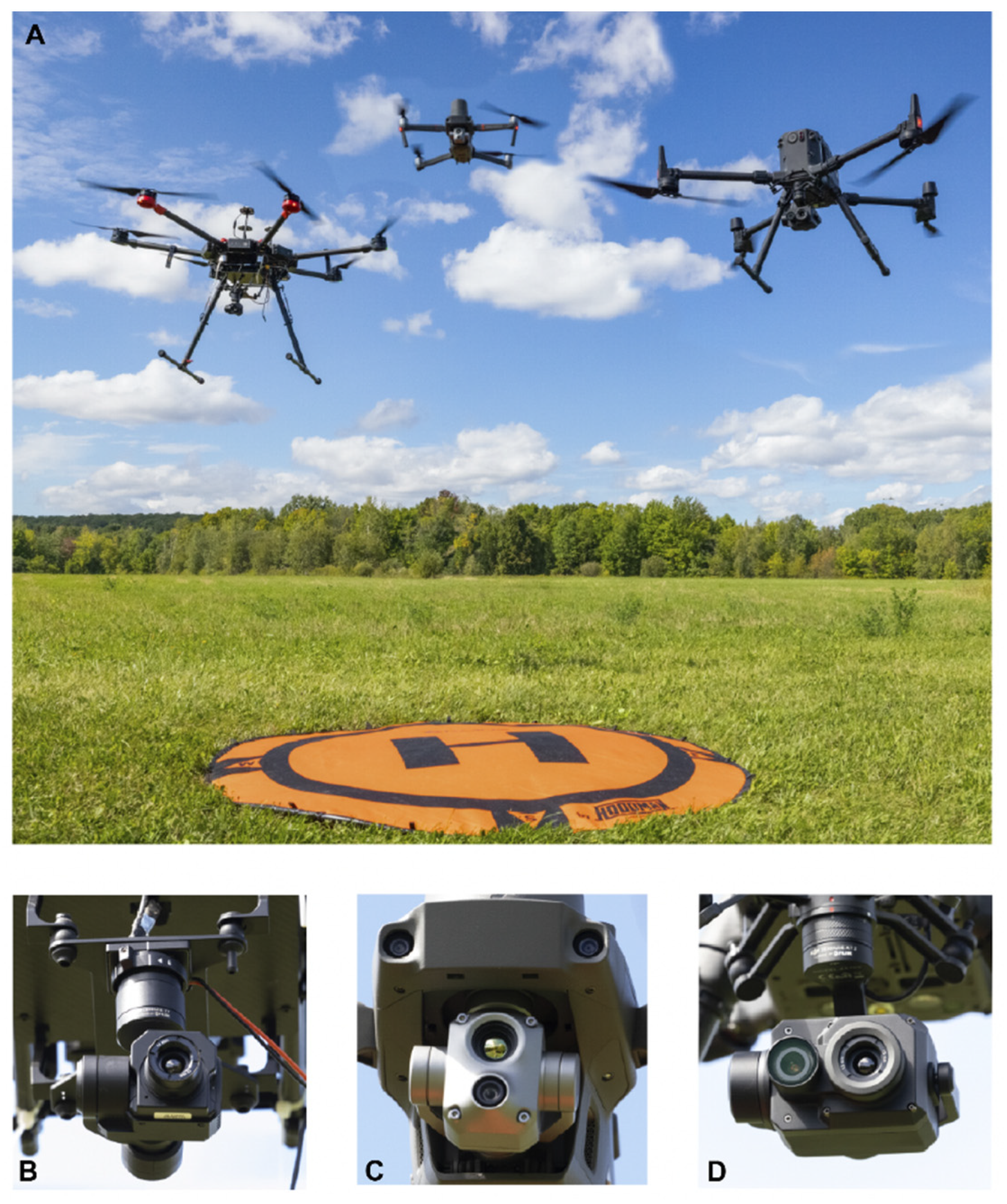
Da-Jiang Innovations, Shenzhen, China (most commonly referred to as DJI) is the largest and most popular civilian multirotor VTOL (Vertical Take-Off and Landing) RPAS manufacturer in the world. As of 2019, DJI systems comprised 76.8% of the market in the USA (based on FAA registrations) [40]. As such, we have chosen three DJI RPAS models with TIRI capabilities, they are: the Mavic 2 Enterprise Advanced (hereafter M2EA), the Matrice 600 Pro (hereafter M600P) and, the Matrice 300-RTK (hereafter M300) (Figure 1). Table 1 contains general physical [41,42,43] and costing information for each of the RPAS airframes.
The M2EA airframe is the only one of the three tested here that has the dual TIRI/visible camera and gimbal system form-integrated into its airframe. Therefore, unlike the M600P and the M300 airframes, the M2EA is not suitable for interchanging with other camera systems. Both the M2EA and M300 geotag the thermal images with RTK (Real Time Kinematics) corrected positional information, which allows for accurate (<3 cm horizontal) geopositioning [44]. However, because it does not use a local base station, in order for RTK to be enabled on the M2EA, an external cellular internet connection and incoming corrections are necessary. While the M600P uses the RTK module in differential mode for flight control, the geotags of the XT-R are based on the basic GNSS (Global Navigation Satellite System) position.
Unlike the M2EA, the M600P and the M300 airframes are able to carry a wide range of payloads, including various TIRI systems and gimbals. This is due to their payload carrying capacity—up to 11.5 kg and 2.7 kg, for the M600P and M300, respectively. The M600P and the M300 airframes are also more robust than many similarly classed airframes in terms of general physical presence, flight endurance and having a wider operational envelope. The M300 has an Ingress Protection (IP) rating of IP45, meaning it is protected against solid objects that are >1.0 mm in diameter, and also from water coming from any direction.
As this study is focused on TIRI for RPAS, we have selected DJI’s M2EA, the Zenmuse XT-R and the Zenmuse XT2 cameras for comparison. We distinguish the XT-R (radiometrically calibrated) version from the non-calibrated performance version not tested here. Standard specifications of each camera is shown in Table 2 [41,45,46]. The XT2 is the only camera tested that has an Ingress Protection (IP) rating (IP44), which indicates that it is protected from solid (i.e., dust) and water particles/drops larger than 1 mm. Considering that these cameras are some of the most popular models for RPAS TIRI, the outcome of this comparison is expected to bring some insight into the potential impacts that newer/older, smaller/larger and, expensive/cost-effective technology may have on the quality of data produced. For greatest accuracy of measurement, all three cameras are recommended for use by the manufacturer in applications where the emissivity (see Section 2.2.1) of the material under study exceeds 0.9. All three cameras have high and low gain modes; in this study, all data were acquired in high gain mode to increase sensitivity (at a loss of the overall usable scene temperature range).
2.2. Blackbody Indoor Camera Validation
2.2.1. Thermal Radiation
In considering the thermal behavior of a material, it is very useful to invoke the construct of a “blackbody”—a theoretically perfect radiator that absorbs all incoming energy (no reflection) and, when in equilibrium, becomes a perfect emitter. Therefore, when in thermal equilibrium, a blackbody is both a perfect absorber and emitter of incident radiation. An important quality of the surface is that it is perfectly isotropic, emitting and absorbing incident radiation without directional bias.
To understand the blackbody energy relationships of interest to this study, we begin with Planck’s blackbody radiation law (Equation (1)), which describes the intensity of the electromagnetic radiation emitted by a blackbody at a given wavelength as a function of its temperature,
where, Iλ is the spectral emissive intensity (W∙m−2∙sr−1∙µm−1) of the radiation emitted by the blackbody at a given wavelength, λ (in µm), T (in kelvin) is the absolute temperature, h is Planck’s constant (6.626 × 10⁻³⁴ J∙s), c is the speed of light (2.9979 × 10⁸ m∙s−1) and k is the Boltzmann constant (1.380649 × 10⁻²³ J∙K−1).
In work with electromagnetic sensors and imaging systems, one of the main quantities of interests is the energy at which a system radiates. Therefore, with Equation (1) as a basis, the total emitted radiation (E) of a thermal system is well-known to be a function of the temperature associated with the body and is given as:
where, σ is the Stefan–Boltzmann constant (5.670374 × 10⁻⁸ W∙m−2∙K−4) [47]. Equation (2) shows that there is a relatively simple relationship between the temperature of a body and the energy of that body and that it is proportional (by the Stefan–Boltzmann constant) to the 4th power of the temperature. The important behavior that Equation (2) is able to determine is that a change in temperature within a system (a body) produces a large change (relative to the magnitude of the temperature change) in energy output for the system.
While Equation (2) is certainly useful in many respects, for this work, we are primarily interested in a subset of wavelengths due to the fact that imagers have a finite sensitivity over specific wavelength ranges (7.5–14 μm in our case—from Table 2). Fortunately, there is a well-known derivation (Wien’s law) of Equation (1) that determines the wavelength at which the maximum radiant energy (λmax) is produced as a function of temperature, and is given below as:
where, b, is Wien’s constant (2.8978 × 10⁻³ m∙K). We note that while Equation (3) determines the maximum, or peak, wavelength, it cannot be forgotten that there remains a continuum of wavelengths produced from a body, at temperature T above 0 K. This continuum is fully described by Equation (1) and is the blackbody curve for that temperature.
Although the construct of a perfectly emissive radiator (blackbody) is well-defined, real-world materials deviate from this perfect behavior by emitting less energy than that predicted by blackbody theory. This deviation is captured by the emissivity coefficient (ε) and is quantified as the ratio of the energy emitted from a material’s surface (Em) to that emitted by a blackbody (Eb):
Emissivity is a unit-less characteristic of real-world materials that is dependent on several factors including: wavelength, temperature, material composition and surface characteristics (including, roughness, angle and direction). It is the most important factor of a surface that affects the amount of energy radiating from it [48]. The closer the value of ε is to 1, the greater is that material’s thermal behavior approximating that of a blackbody. Accordingly, objects with high ε absorb and radiate large amounts of energy, while those with low ε, such as most metals, absorb and radiate low amounts of energy but are highly reflective. Therefore, in order to retrieve accurate surface temperatures of real-world materials, it is fundamentally important to correct for the ε of the materials. In general, when collecting the raw TIRI data, the radiative temperature is often acquired and expressed as Brightness Temperature (BT). The BT represents the temperature that a blackbody would be at in order to generate the observed radiance at the given wavelength (as ε = 1 in this case). It is important to note that BT produces incorrect surface temperatures for real materials; therefore, it is necessary to apply the correct emissivity value (from Equation (4)) in order to determine the true surface temperature of a material.
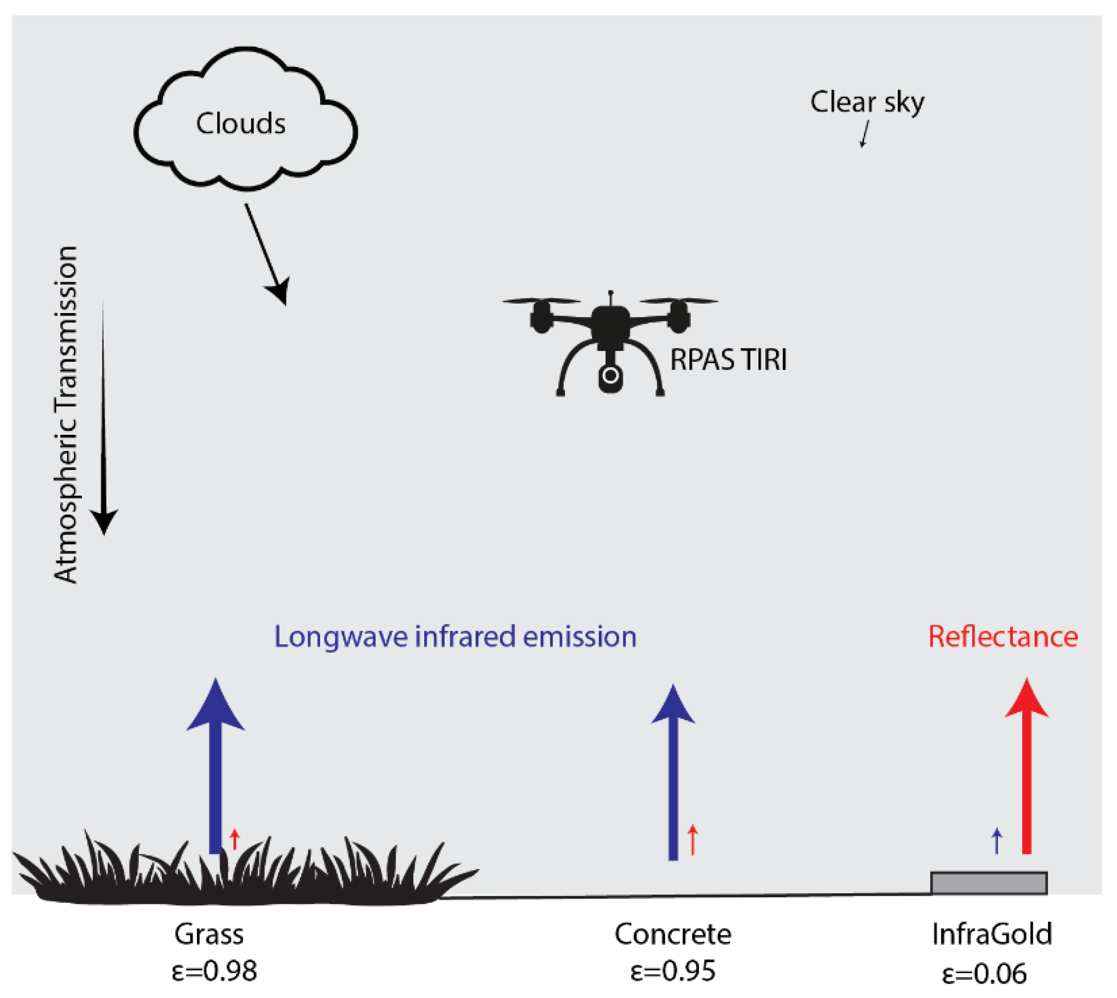
While emissivity is certainly important, there are also energy contributions from a number of other factors that need to be taken into account with typical RPAS TIRI estimations of surface temperature (Figure 2). As an example, sky/cloud contributions heavily depend on the condition (i.e., percent cloud cover and cloud type) with clear skies contributing the least. In contrast, thick cumulus clouds contribute considerably more energy to the measurement [49].
2.2.2. Indoor Camera Validation—Blackbody Radiator
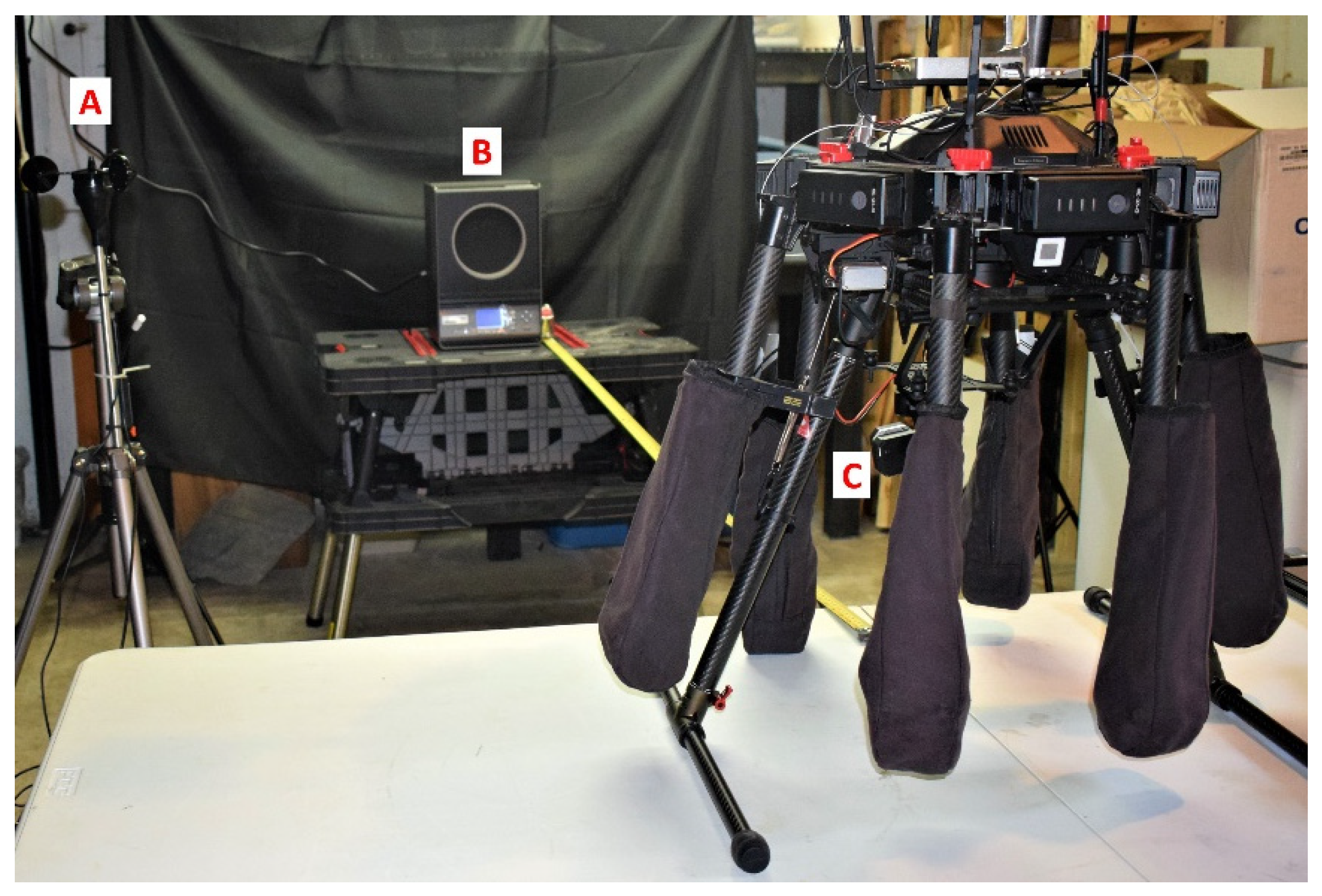
While it is often the case that small RPAS radiometric TIRI cameras come with a factory calibration certification, it is important (often necessary in practice) to validate if the calibration remains accurate at or near the time of the survey. The two primary reasons are that, (1) often there has been some physical jarring action during transport, which can potentially cause the unit to become uncalibrated and (2) all camera systems are not created equal, with quality greatly differing between them. The validation of TIRI systems involves the use of a stable calibrated blackbody source. In this study, we used the FLUKE 4180 Calibrator (Fluke Corporation, Everett, WA, USA) [50] as the target source for the validation. The FLUKE 4180 is a well-known portable blackbody operating within the −15 °C to 120 °C temperature range with a large 15.24 cm diameter target radiator. Over the temperature range of this work, the calibration error was 0.4 °C (obtained via the instrument’s calibration certificate) at each temperature measured. The unit has a stability of +/−0.05 °C and +/−0.10 °C at 0 °C and 120 °C, respectively. Over the central 12.7 cm diameter of the target, the radiator has a uniformity of +/−0.1 °C and +/−0.20 °C at 0 °C and 120 °C, respectively. The unit has a nominal emissivity of 0.95 but is applicable over the range of emissivities (0.9 to 1.0) via thermometer emissivity compensation. As it was calibrated for ε = 0.95, all the imaging measurements for this work have used the 0.95 nominal emissivity value. As per the instructions of the manufacturer, the unit requires 10 min of settling time after reaching the desired testing temperature to ensure the stability of the target radiator. Figure 3 shows the set-up of the indoor validation exercise.
The motivation of this validation process was to set the blackbody source at a distance away from the cameras that is greater than the minimal focal distance of the camera (for the XT-R and XT the minimum focus distance is 7.6 cm and ~3.2 cm for the M2EA [41,45,46]). Then set the temperature of the blackbody and let it settle to ensure uniformity. After settling, image the blackbody source with the central pixels of the camera and then go to the next temperature, let settle and image—repeat as per necessary for the temperature range expected by the phenomena under investigation. Then, to ensure the instrument and related software are properly accounting for distance, we doubled the distance and re-image at the same temperatures. In this process, we have used the central pixels as they are often (but not always) the ones of concern when we investigate any phenomena. This method, of course, is not entirely complete as the non-central pixels do not image the blackbody; however, we are proposing a realistic method to field-validate RPAS imagers. In order to fully validate the imager, each pixel of the imaging camera should image the central area of the blackbody target. Since we are interested in field-applicable methods, and our imager is 640 × 512 pixels, it is not at all practical (to the RPAS operations) to test more than the central pixels.
We set-up air temperature, pressure, humidity and air speed monitors within the indoor space using the HOBO™ (Honest Observer By Onset) smart sensor system (Onset Computer Corporation, Bourne, MA, USA). The HOBO system is a well-known and highly used suite of field-proofed environmental measurement instruments [51,52,53,54]. During the entire time of the exercise, there was no measurable flow of air, which was not unexpected as we performed this work indoors with no forced air circulation. However, it was necessary to ensure this wasthe case.
Each RPAS camera was positioned at 2 m distance to the blackbody and normal (90°) to the center of the face of the radiator target, so that any angular dependence of measurement was fundamentally restricted to being perpendicular to the measured surface. We then allowed the blackbody to come to the first temperature (5 °C) and once at that temperature, we let it stabilize for 10 min. With each camera in succession, the blackbody radiator target was imaged with the central portion of the camera’s FOV. The blackbody temperature remained constant at the set point while the camera was moved to 4 m from the blackbody target and then each camera re-imaged the blackbody target again. The use of two distances (2 m and 4 m) was an exercise to determine if there were considerable differences in measured temperature as a function of distance, even though each camera has a small focal length of 9 mm (M2EA) or 13 mm (XT-R and XT2). Once all cameras had imaged the blackbody target at both distances for each temperature, the temperature was increased to the next setting and the process was repeated. We selected eight temperature settings (5, 10, 15, 20, 25, 30, 35 and, 40 °C), over a range of 35 °C, that are uniformly spaced and would replicate the air and target temperatures expected in real-world environmental applications. As well, this process ensures the evaluation of the camera performance near to, and including, temperatures beyond those of interest to the application. In our case, the application temperatures of interest were from 15 °C to 25 °C.
The indoor blackbody validation data were acquired over a period of 2.5 h, after set-up, where the majority of that time was dedicated to allowing the blackbody target radiator to settle after reaching the testing temperature. Once the temperatures were recorded by the TIRI cameras, the images were processed in FLIR Thermal Studio (Teledyne FLIR, Wilsonville, OR, USA) in order to account for emissivity, distance to source, air temperature, humidity, and optics temperature. As the images from the M2EA cannot be directly read by FLIR Thermal Studio, they were first converted to a standard FLIR radiometric jpg with ThermoConverter (Aethea, London, UK).
2.3. Outdoor Field Trial
2.3.1. Study Site Set-up
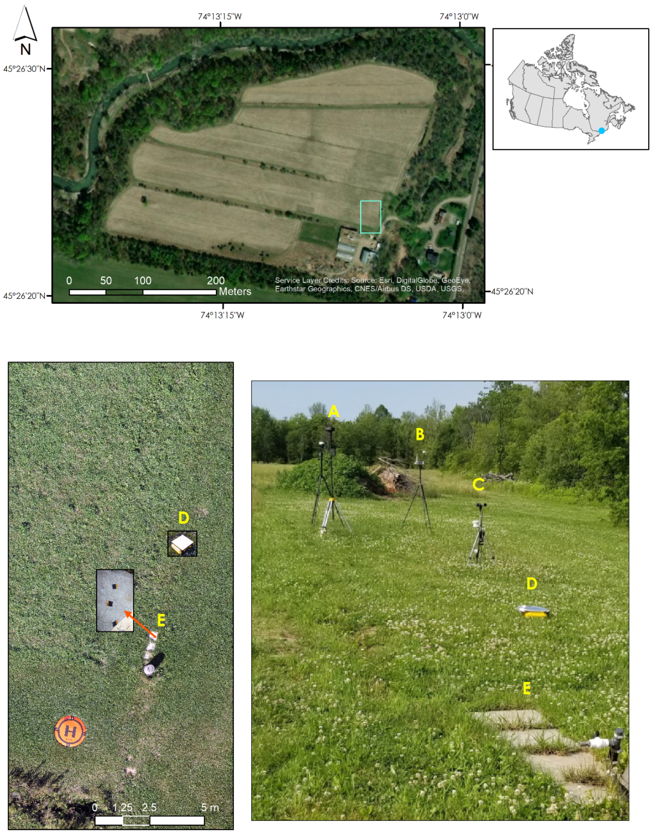
The location of the field trial was at a private RPAS test site near Vaudreuil-Dorion, QC, Canada (45°26′23″ N, 74°13′05″ W). The extensively instrumented ground site is shown in Figure 4. The ground site set-up and the instrument distribution included: 2 differential RTK base stations supporting the M300 and M600P, HOBO environmental measurement station, vegetation validation targets, an InfraGold target panel and, concrete slab validation targets. The RTK base stations were used during the trial to replicate flight conditions appropriate to larger area TIRI acquisitions.
The HOBO environmental monitoring instrumentation (Figure 5) consisted of measuring the following (with model numbers): an anemometer (S-WSA-M003) for measuring wind speed, and wind gust, air temperature (Tair) and relative humidity (RH) ((A-THB-M002), solar shielding (RS3), air pressure (S-BPB-CM50), two in-canopy vegetation temperatures (S-TMB-M006), and two soil temperature probes (S-TMB-M002). The electronics and data collection units (H21-USB) were stored under the tripod. Tair and RH are integrated into one unit (S-THB-M002), and were placed under the solar shield (RS3) in order to obtain accurate Tair and RH measurements free from the effects of direct solar radiative heating [51].
While, Tair will have a large impact on surface temperature, wind speed has been shown to induce substantial localized cooling depending on its value over a sustained period of hours. Wind-induced surface cooling arises as a case of forced convective cooling and is proportional to the temperature differential between the air in motion and the surface [55]. Several studies using TIRI have shown and measured this effect on surfaces of buildings [56,57], and on the bare ground overtop of heating pipe systems [58]. In general, these studies show that with wind speeds below 2 m/s the effect is negligible, or at least at the limit of the resolution of the TIRI data. The work of [58] remains as one of the few examples of TIRI-derived temperature measurement as a function of increasing wind speed. In [58], TIRI taken overtop of buried heating pipes have shown that winds below ~2 m/s did affect the measurements but the value of this effect (~+/−0.2 °C) is less than the error in the TIRI data. In more recent work, [56] found that for many building surfaces, winds up to even 5 m/s did not significantly alter the values obtained via a TIRI survey. In an even more recent work, [57] generalized that wind pulsations (gusting) induced changes with TIRI data as being “not-critical” for speeds of up to 2 m/s. Sustained wind periods of several hours before data collection did have an impact on the surface temperature and should be avoided during those times. As a result of this known wind-induced cooling, the majority of past studies identified that it is often necessary to install the environmental monitoring equipment (Figure 5), at least several hours before TIRI data collection.
Figure 6 shows the three targets of interest for this study, the InfraGold panel, the concrete slabs and, the in-canopy vegetation and soil targets. The diffuse InfraGold panel (25.5 cm × 25.5 cm), is being used only to determine if there is a significant contribution to the signal from the downwelling irradiance of the open sky [49]. Having an ε = 0.06 means that it is highly reflective and as it faces the sky, the conditions it presents to the imager is that of the sky with negligible contribution from its own emission (i.e., less than the detection limit of the TIRI camera) at most ambient air temperatures at which RPAS TIRI is carried out.
The patio stone concrete target, Figure 6B, were in place for several years prior to the experiment and, therefore, was in good contact with the underlying soil. The surfaces of the concrete slabs were weathered. Three FluxTeqTM PHFS-01-e 1 × 1” standard heat flux sensors (Flux Teq, Balcksburg, VA, USA) were connected to a high resolution, 8 channel thermocouple data acquisition device (TC-DAQ) logging to a laptop. The PHFs-01e have a nominal sensitivity of 9.0 mV/(W/cm2) and a specific thermal resistance of 0.9 K/(kW/m2) [59]. The PHFs-01e heat flux sensors were adhered to the concrete using Arctic MX-4-4G thermal compound paste (carbon micro-particle based) (Arctic GmbH, Braunschweig, Germany). One of the three flux sensors did not properly adhere to the surface of the concrete, and thus those data were ignored in this study.
The soil and in-canopy temperature sensors were configured to work in pairs where the soil temperature probes were placed directly below the in-canopy temperature probes at a depth of 5 cm from the surface. In our set-up, shown in Figure 5E and in detail in Figure 6C, the T1 and T2 sensor pair was located 1 m north of the middle of the anemometer tripod. The in-canopy sensor (T1), located by the red arrow in Figure 6C, was held in place by a nylon cord that was attached to wooden stakes driven into the ground approximately 5 cm on either side of the sensor. This was necessary as curious field animals have a tendency to remove these sensors when left in place overnight. The other pair of in-canopy and soil temperature sensors, respectively, T3 and T4, were installed in the same manner, 1 m south of the anemometer tripod (location F in Figure 5). The vegetation target area is composed of a heterogeneous mix of grasses, white clover, dandelion and detritus, as well as void space. The overall result is that the soil is fully overlaid by the living vegetation canopy and its detritus. At the time of the TIRI measurements, the height of vegetation was ~10 cm. The soil and in-canopy sensors were installed and logged continuously for 12 days prior to the acquisition of the RPAS TIRI images.
2.3.2. RPAS TIRI Acquisition
The TIRI RPAS measurements were made after twilight (21:25 EST) on 5 July 2021 in order to ensure that solar irradiance would not influence the measurements. For a large amount of TIRI work, it is highly desirable to work after twilight in order to eliminate the potentially large non-linear differential solar contribution to the measured signal (Holtz 2000). For the TIRI acquisition starting at 10 m height above the study area, the first RPAS airframe hovered over the targets and acquired a thermal image—manually triggered by the operator. It then ascended to 20 m and repeated the acquisition. In this manner all three airframes completed the acquisition of the TIRI at heights of 10, 20, 30, 40 and, 50 m. The multi-altitude data set was acquired over a period of ~30 min. Even though each of the thermal cameras carry out flat field corrections (FCC) at power up and periodically during use, a supplemental FCC was triggered by the operator prior to the acquisition of each image. The FCC compensates for errors that occur during operation—such as those induced by temperature change at altitude. The images were processed in FLIR Thermal Studio to account for height (i.e., distance from target), atmospheric temperature, relative humidity and reflected temperature. The external optics temperature was set to Tair recorded at the time of acquisition. The images were processed with three different emissivity values, 1 for BT, 0.98 for grass and 0.95 for concrete. As with the blackbody radiator experiment, the M2EA images from this test were also first converted to a standard FLIR radiometric jpg with ThermoConverter.
In this work, we have used the value of ε = 0.98 for vegetation, which is based upon [60] (as cited in [61]) who have suggested this value for a general canopy emissivity. The value is further supported by [62] who have described grass emissivities for complete and partial canopy covers ranging from 0.956 to 0.986. More recently, [16] have used ε = 0.979 for grasses and ε = 0.977 for canopy cover, and [61] used ε = 0.98 as the vegetation canopy emissivity in non-arid environments. The emissivity value used for concrete (grey weathered, rough surface) was obtained from [63] where a large number of urban materials have undergone emissivity determination within the 8–14 μm range.
3. Results
3.1. Indoor Blackbody Validation
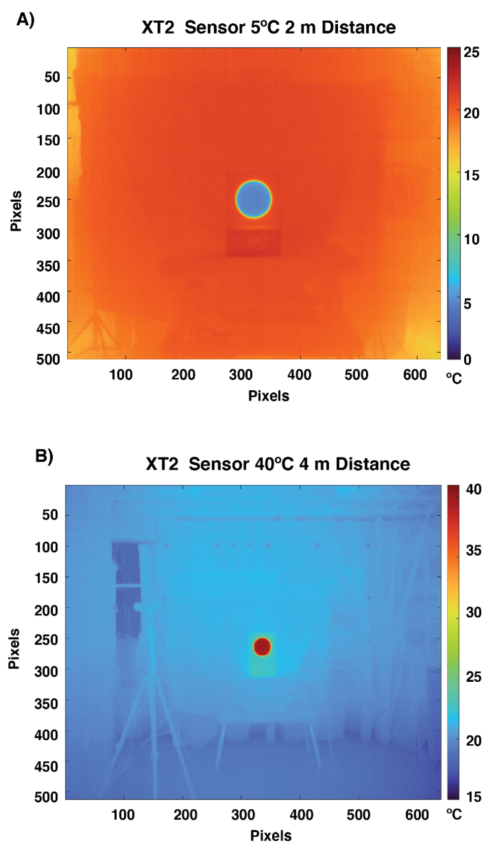
During the indoor trial, the environmental parameters were reported as: Tair average of 20.6 °C (ranged from 20.2 °C to 21.0 °C), RH average of 70.9% (ranged from 69% to 71.7%) and barometric pressure average of 1009.2 mbar (ranged from 1008.5 mbar to 1009.9 mbar). For the purposes of this work, we used the average Tair, pressure and RH for the calculation of the environmental temperature, in the vicinity of the blackbody, by each camera. The imagery obtained from each camera showed that the blackbody radiator target was well identified at each of the eight temperature settings. Examples of the imagery are shown in Figure 7 for the XT2 camera, at 2 m and 4 m distance, for 5 °C and 40 °C, respectively. The pixels in the central portion of the blackbody radiator (all within the 12.7 cm diameter of the central area of the radiator) were used in the subsequent analysis of the temperature measurements. The portion of the image outside of the area of the circular blackbody radiator exhibits less detail (lower contrast) as the material within the room was at or near the average indoor ambient temperature of 20.6 °C. A total of 830–950 pixels comprised the area extracted for analysis at 2 m and 220–230 pixels at the 4 m distance.
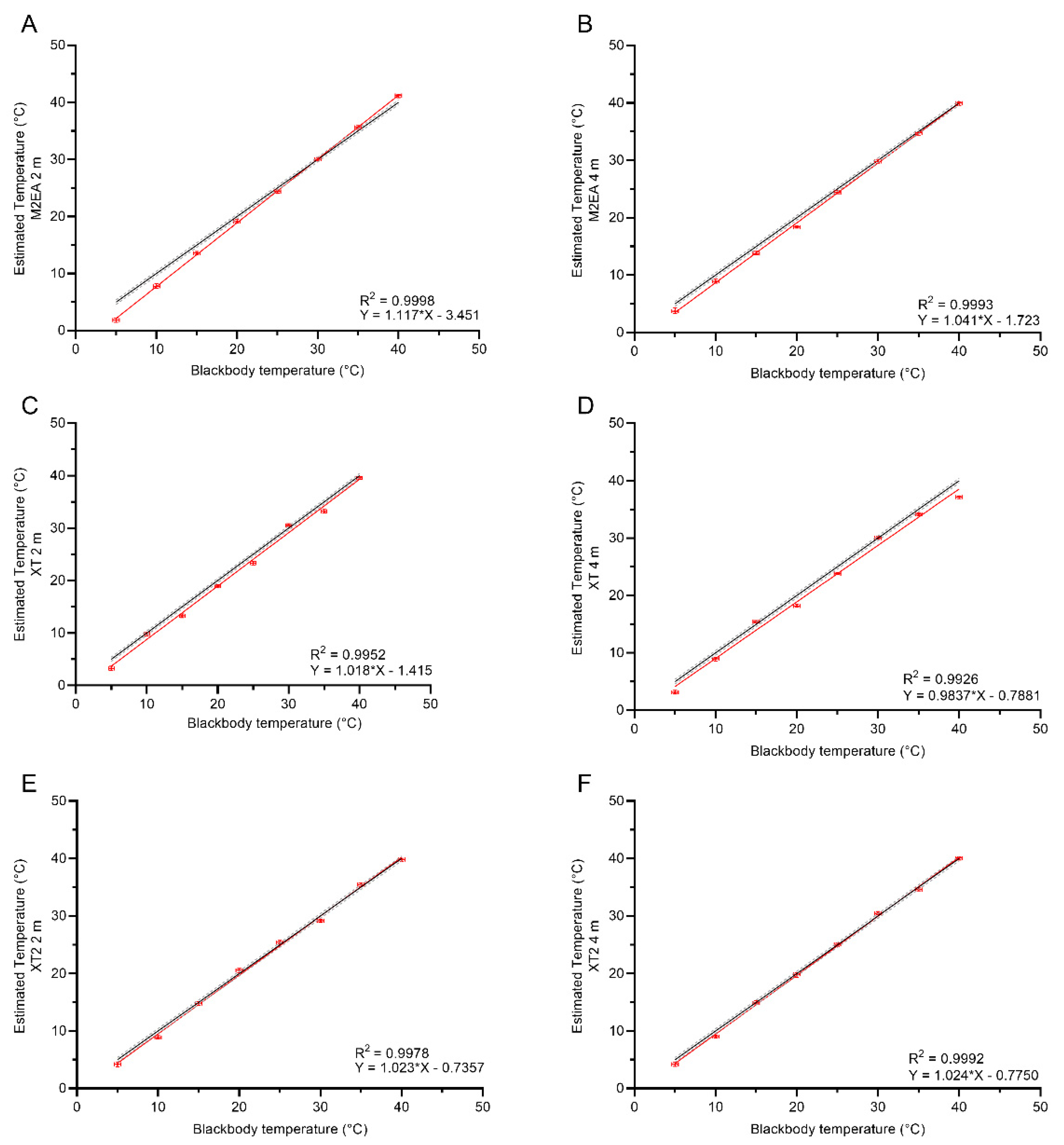
The measured results for each camera at all temperatures and distances, are shown in Figure 8 along with the best fit lines and uncertainties related to the measurements. The data used for Figure 8 is provided in Table A1 in Appendix A. The error bars shown for each plot arise from the range (minimum and maximum values of the central pixels) of the measurements themselves. Also presented in each plot is the corresponding 1:1 temperature line (black solid) that represents the theoretically perfect blackbody target temperature and the uncertainty (black dashed lines) corresponding to the +/−0.4 °C uncertainty value that was supplied by the calibration certificate. For each data set shown in Figure 8, statistical analytics describing the linearity of the response and the deviation from the blackbody source are shown in Table 3.
Overall, Figure 8 shows that each camera is highly linear over the temperature testing range of 5 °C to 40 °C. The linear relationship for each camera shown in Figure 8 is reflected, numerically, in the results of Table 3 with each best fit line having an R2 > 0.99 The 95% confidence intervals of the slope for the M2EA at both distances are the only ones that do not span 1.0 (i.e., slope of the 1:1 line) substantiating the larger underestimation of the blackbody temperatures of 5 °C and 10 °C see in Figure 8A,B. Over the temperature range investigated with the blackbody (35 °C), the M2EA had the greatest temperature difference (ΔT) (36.2 °C at 2 m and 39.3 °C at 4 m) from the ΔT of the blackbody (35 °C). In contrast, the XT2 had the least difference with a ΔT of 35.8 °C and 35.6 °C at 2 m and 4 m, respectively. The standard deviation for the measurements at each temperature was less than 0.15 °C for all cameras indicating a consistency in pixel values across the imaged surface of the blackbody (Table A1).
The analysis results for each camera at each distance are summarized in Table 3 and indicate that all cameras, in general, underestimated the blackbody temperatures. At the 2 m distance, the greatest deviations in the measured temperatures were found to be −3.1 °C and −2.2 °C for the M2EA at blackbody temperatures of 5 °C and 10 °C, respectively. At the 4m distance, the XT-R camera had the greatest deviations from the blackbody with −2.9 °C and −1.9 °C at 40 °C and 5 °C respectively (apparent in Figure 8 as well). The largest RMSE values at both distances are seen for the XT-R (0.94 °C and 1.12 °C). It also presents the greatest bias at both distances of −1.00 °C and −1.15 °C (Table 3, Figure 8). Consistently at both distances, the XT2 has the lowest bias (−0.21 °C and −0.23 °C). While its RMSE values were not as low as that of the M2EA (<0.4 °C), they were still less than 0.7 °C for both distances.
3.2. Outdoor Field Trial
Environmental Conditions
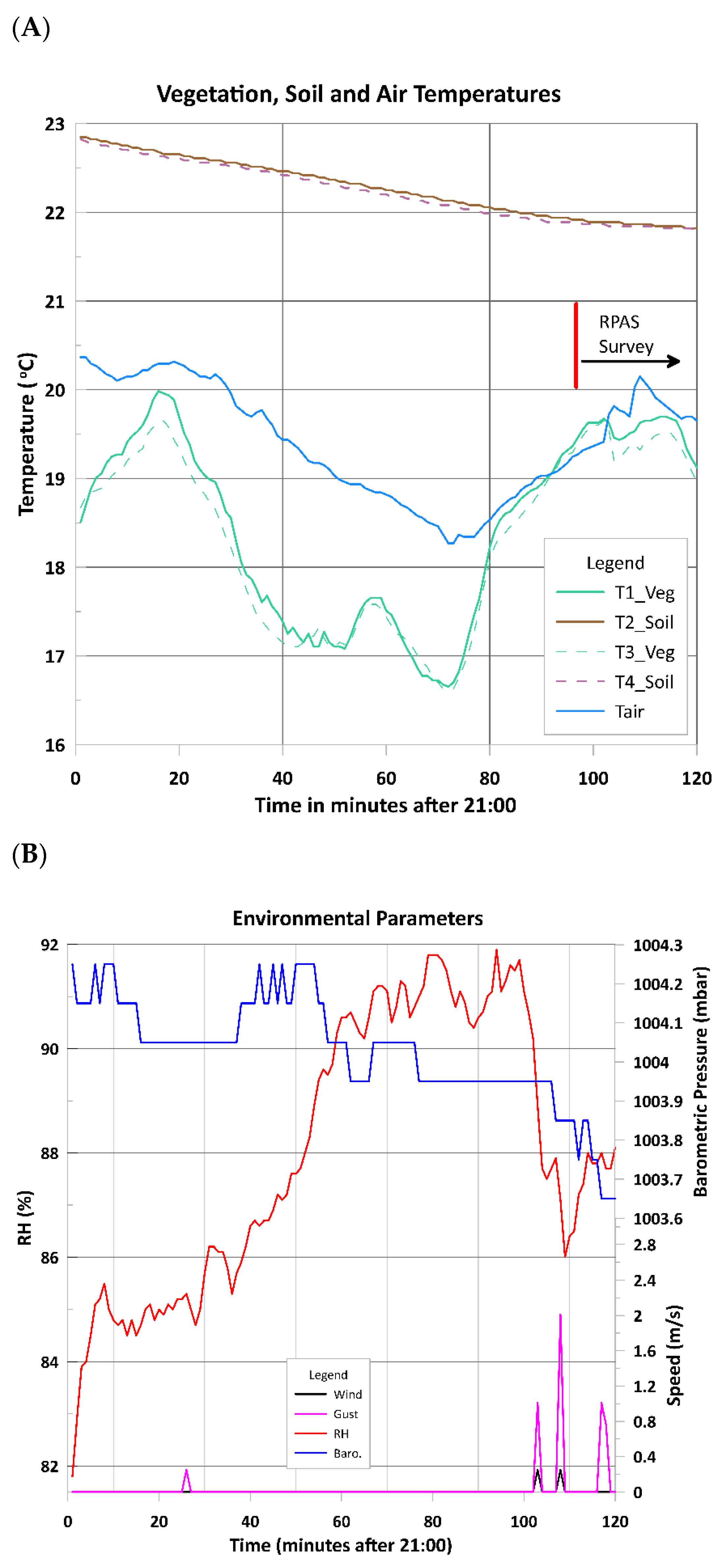
As previously noted, when considering doing TIRI work, the need to collect environmental data (Tair, wind and gust speed, RH, and air pressure) for several hours prior to taking thermal measurements is imperative. In our work, the results of these environmental measurements for the two hours prior to the end of the RPAS TIRI collection are shown in Figure 9 (along with the start time of the RPAS survey). On the day of the survey, twilight occurred at a time of 21:25 EST.
Figure 9A shows the temperature profiles of each sensor that measured the vegetation (T1 and T3), soil (T2 and T4) as well as that of Tair, for direct comparison. As a result, it is clear that variation in soil temperatures (1.0 °C) does not experience the larger fluctuations evident in the vegetation (3.3 °C) or Tair (2.1 °C). The soil profiles (T2 and T4) are also very similar in values, having a maximum difference of 0.07 °C (well within the +/−0.2 °C accuracy of the sensors); they also show a constant cooling slope over the first 90 min and again over the last half hour of the trial period (~2 h). The small change in cooling slope for the soil is likely due to the delayed effects of the increasing Tair and vegetation temperatures. A similar relationship to soil exists for the vegetation sensors (T3 and T4) where they mimic each other’s profiles, however, there are differences that amount to ~0.7 °C (nearly 10 times that of the soil profiles) which is larger than the error of the sensors and is therefore, real but still quite small. T1 and T3 also mimics Tair (with some offset in time and a larger offset in temperature) but to a lesser degree. It is also evident that Tair has the most influence on the variability of T1 and T3; moreover, during the time of the RPAS survey (shown in Figure 9A), Tair, T1 and T3 experience ~0.5 °C of variability, which will be considered as remaining essentially constant for the duration of the survey.
For the environmental factors in Figure 9B, the time during the RPAS TIRI data collection period shows small amounts of variability—with barometric pressure varying by 0.2 mbar and RH by 5.9%. Therefore, we are treating these parameters as being essentially constant for the purposes of calculating source temperatures from TIRI. In this study, the wind and gust averages for the 2 h prior to the end of the trial were 0.01 m/s and 0.03 m/s, respectively—well below the 2.0 m/s value where they would start to influence the surface temperature measurements. Moreover, the maximum gust speed obtained was 2.0 m/s for a single point anomaly (at time point 108 in Figure 9B). Under these conditions, we can confidently say that the wind had no effect on the targets of interest.
While the environmental parameters in this study have been shown to be essentially constant or insignificant, it is important to measure the variables, in situ [14], as it could easily have been the case that the conditions exceeded the bounds of influence for TIRI temperature retrieval. Furthermore, the variables of humidity and Tair, along with an assumption of constant and near standard air pressure (1000 mbar), are required input values (or assumptions) for the radiometric correction software.
3.3. TIRI
3.3.1. Brightness Temperature
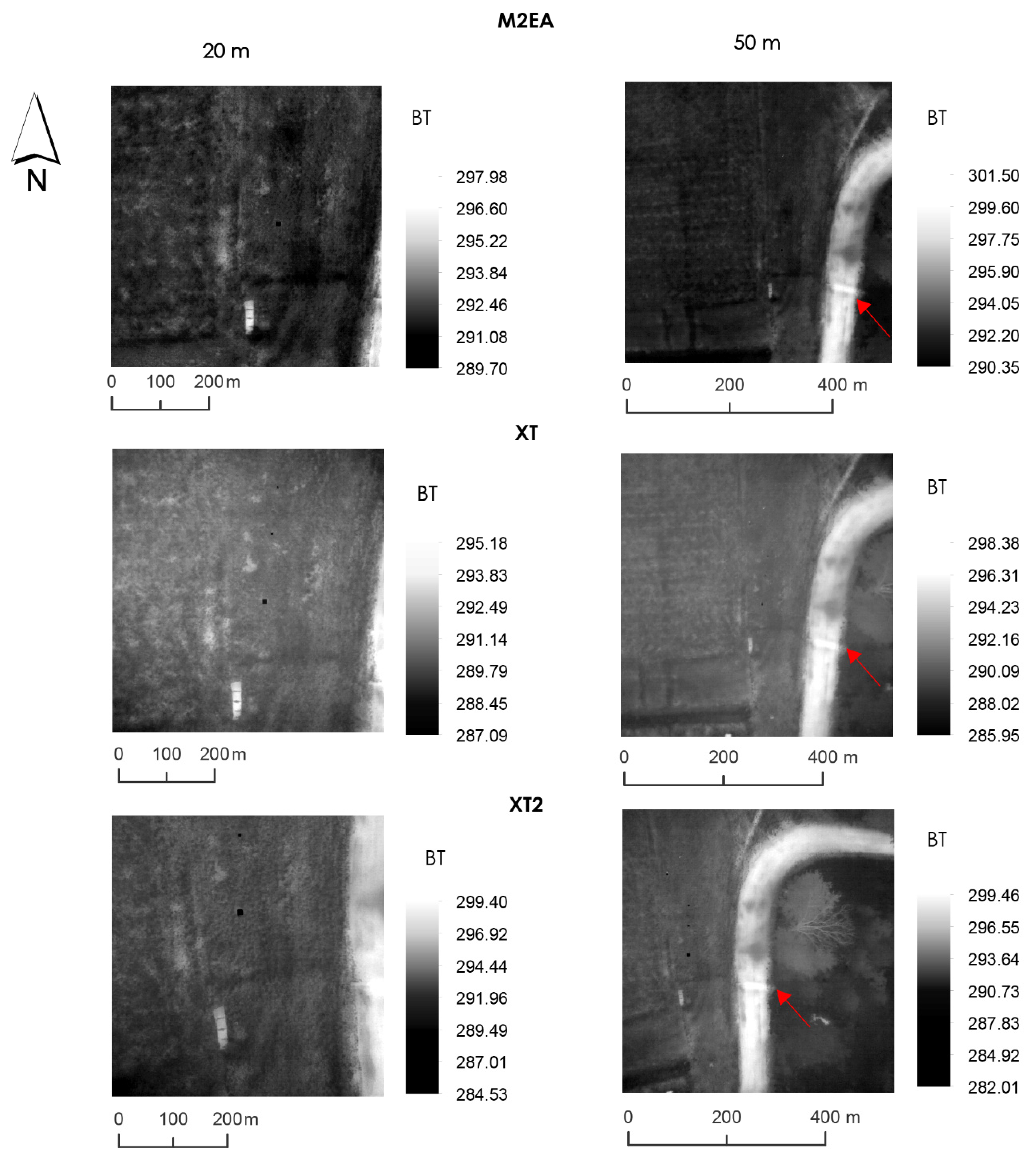
As previously discussed, BT is the collection of TIR measurements with ε = 1. It assumes all radiating surfaces in the scene are blackbodies. While BT is not an accurate measure of surface temperature for real materials, it is useful to compare these values across the scene and for quickly identifying changes in the thermal properties of the area under investigation. The relative differences within the imagery can provide a “quick view” of the potential areas of interest. As an example, Figure 10 shows the results of collecting 20 m and 50 m height TIRI with each camera in this study. It is clear from the 20 m data that all the features we are interested in, (i.e., InfraGold panel, vegetation and, the concrete patio stones), are all identifiable, while the larger area of the 50 m data also shows a curious high temperature linear feature (shown by the red arrow) cross-cutting the direction of the dirt road (brightest feature in the imagery from all three cameras). This feature was later investigated and found to be a buried drainage pipe under the roadway.
3.3.2. InfraGold Panel
To reiterate, the InfraGold panel (ε = 0.06) is used in this study as an indicating tool to determine if the thermal contribution from the sky is, or is not, significantly contributing to the TIRI data. Results from FLIR Thermal Studio of the InfraGold panel derived temperatures (at ε = 0.06) produced open sky average temperatures <−60.13 °C. This value derived for the panel constitutes the lowest temperatures that FLIR Thermal Studio could produce, however, the lowest limit for all three cameras in high gain mode is −25 °C. Therefore, we can only state that the reflected sky temperature from the panel is <−25 °C (as shown in Figure 11) indicating a negligible downwelling contribution. From Equations (1) and (3), the <−25 °C contribution provides a corresponding intensity of <3.85 W/m2/sr/µm at a maximal peak wavelength at ~11.678 μm for the panel surface. Comparing this with an average temperature for the vegetation scene at 19.5 °C, which, through Equations (1) and (3), gives an energy of ~8.79 W/m2/sr/µm at a peak wavelength of ~9.9 μm. In addition, because the 11.678 μm peak is near the edge of the sensors’ measurable response, the effects from the downwelling irradiance are not appreciably impacting this work.
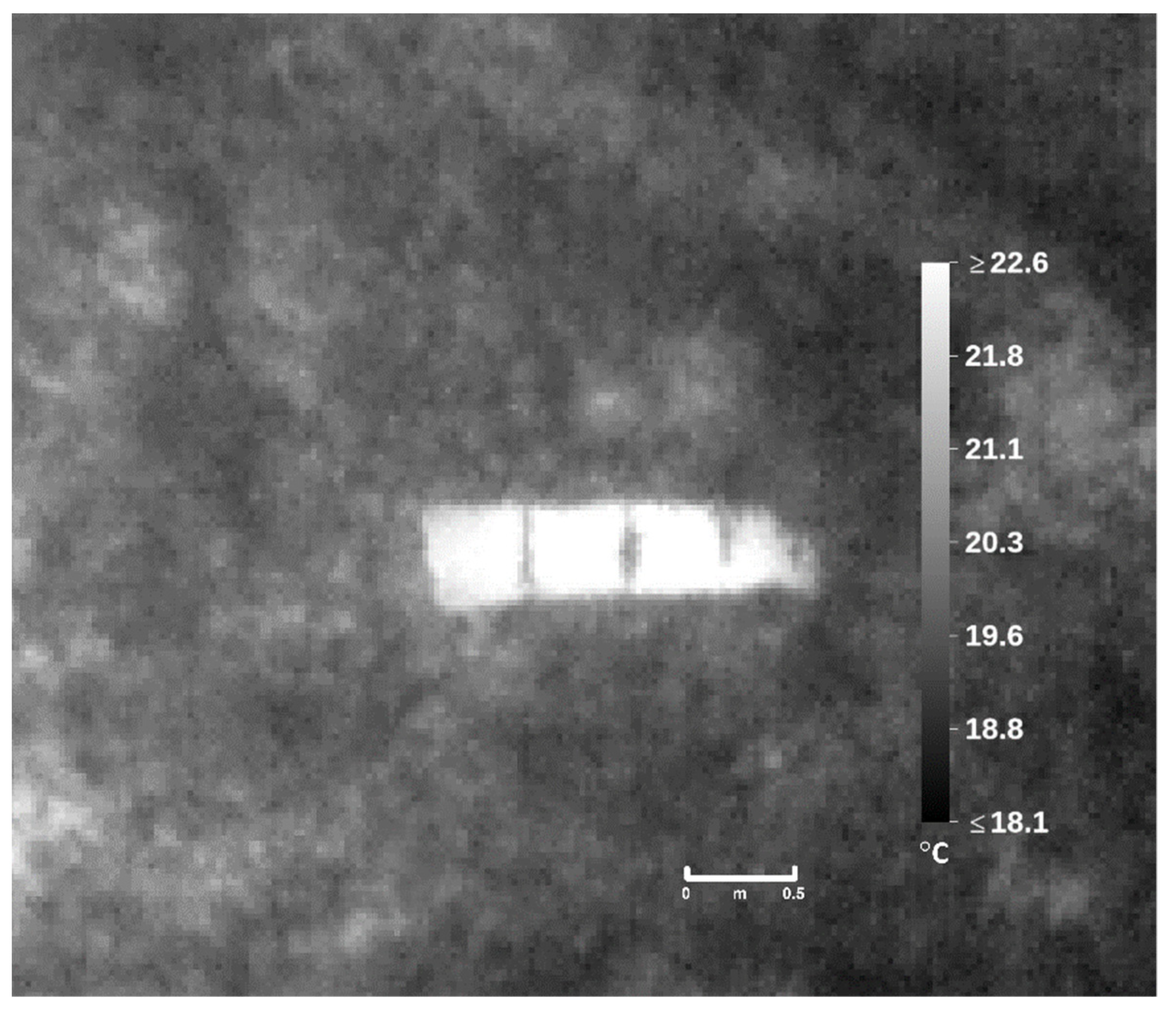
3.3.3. Concrete Patio Stone Target
Figure 12 provides an example of the results of imaging the concrete target with the XT-R camera at 20 m altitude with an emissivity of 0.95. Because of the 41 cm width of the concrete tiles, only the 10–30 m altitude images were included in the analysis. Considering the largest pixel pitch (i.e., 17 µm for the XT-R and XT2) and the 13mm lens, in order to retain the recommended minimum region of interest size of 10 pixels diameter [41,45,46], ensuring accurate temperature retrievals, the sensor/target separation can have a maximum value of 30 m. With fewer pixels, the spot size effect results in lower accuracy measurements due to contamination (spectral mixing) from neighboring materials.
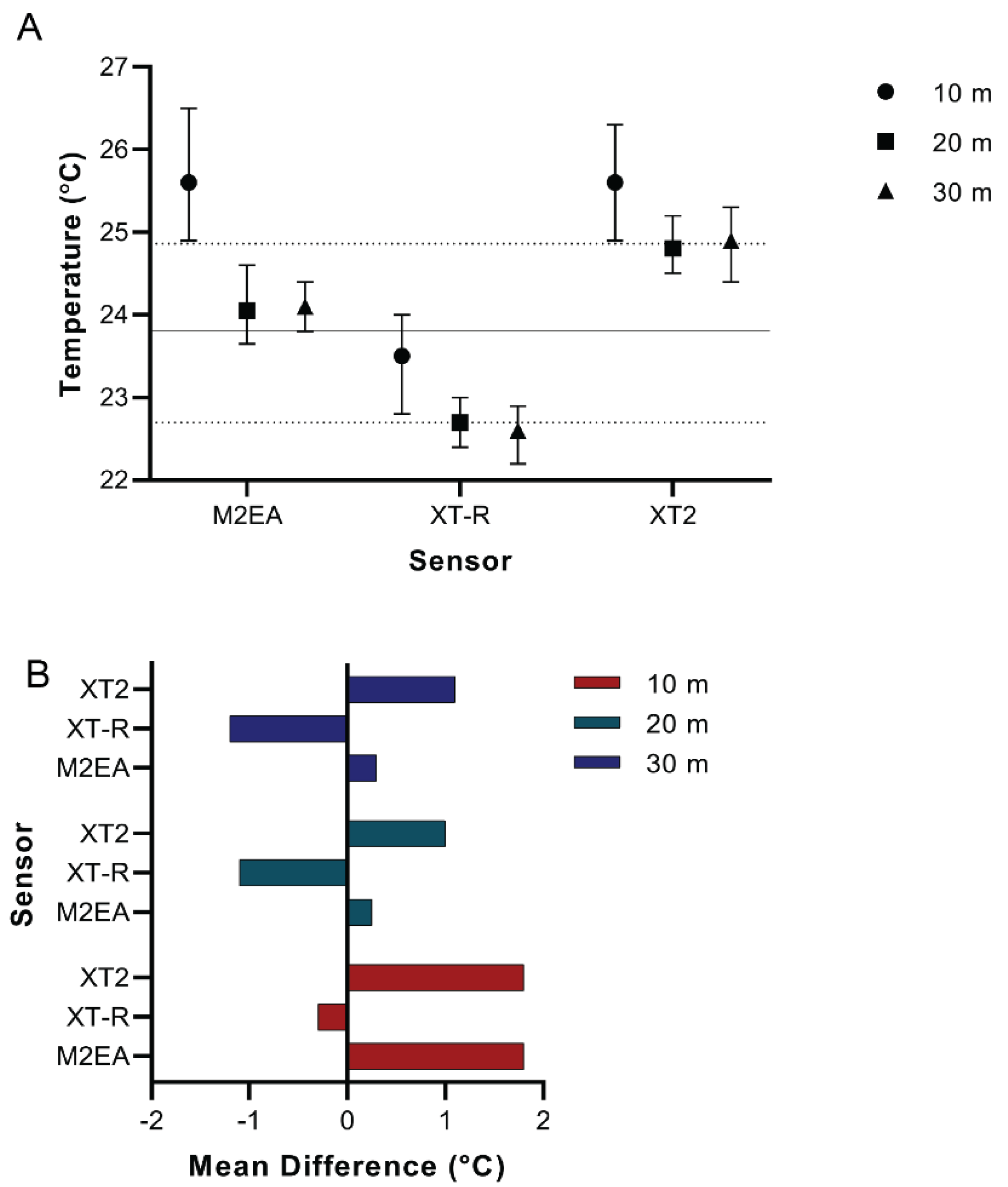
The results of applying the emissivity corrections for concrete to the TIRI data from each camera are shown in Figure 13. The contact measurements from the PHFS-01-e sensors indicated a temperature of 23.8 °C during the data collection. At 20 m and 30 m, the M2EA reports the closest surface temperature to the PHFS-01-e (over estimation of 0.3–0.5 °C.) At the 10 m height, however, the M2EA overestimated the concrete temperature by 1.8 °C. At 20 m and 30 m both the XT-R and XT2 have a similarly large deviation from the in situ measurement, although in opposite directions (−1.1 °C, −1.2 °C for the XT-R and 1.0 °C, 1.1 °C for the XT2). At 10 m height, the XT-R was the most similar to the in-situ temperature of concrete (−0.3 °C difference) in comparison to the M2EA and the XT2, which both overestimated the surface temperature by 1.8 °C. In context, however, while the deviations from the in situ measurements are greater than the bias reported with the blackbody experiment (Table 3), they are all relatively small (<2 °C).
3.3.4. Grass and Soil
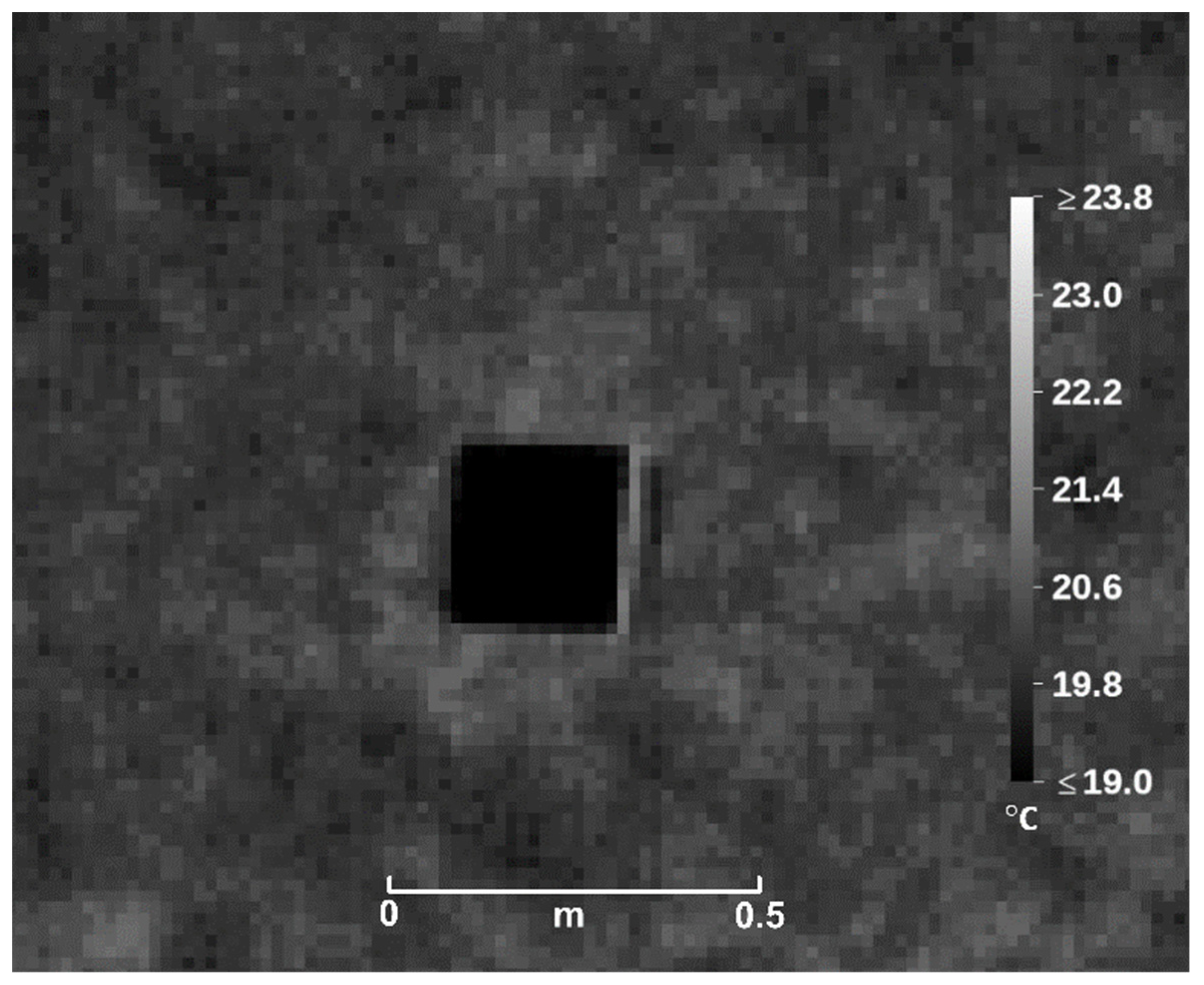
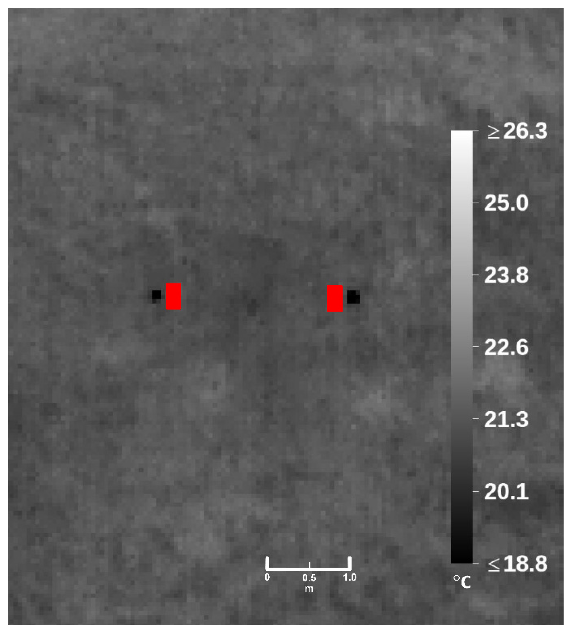
While vegetation targets are complex, due primarily to water content, air space and canopy distribution, they are, nevertheless, important to include as a great deal of outdoor work involves their measure [64,65]. Figure 14 shows an example of a TIRI image of the grass (ε = 0.98) from the XT2 camera at 40 m height. In the image are two black squares (10 cm × 10 cm) of aluminum tape that have been used as markers (due to their very low emissivity- providing high thermal contrast) to locate the areas of the in situ temperature sensors in the resulting TIRI. The markers were placed ~10 cm adjacent to the areas of the in-canopy temperature sensors, bookending the areas of investigation.
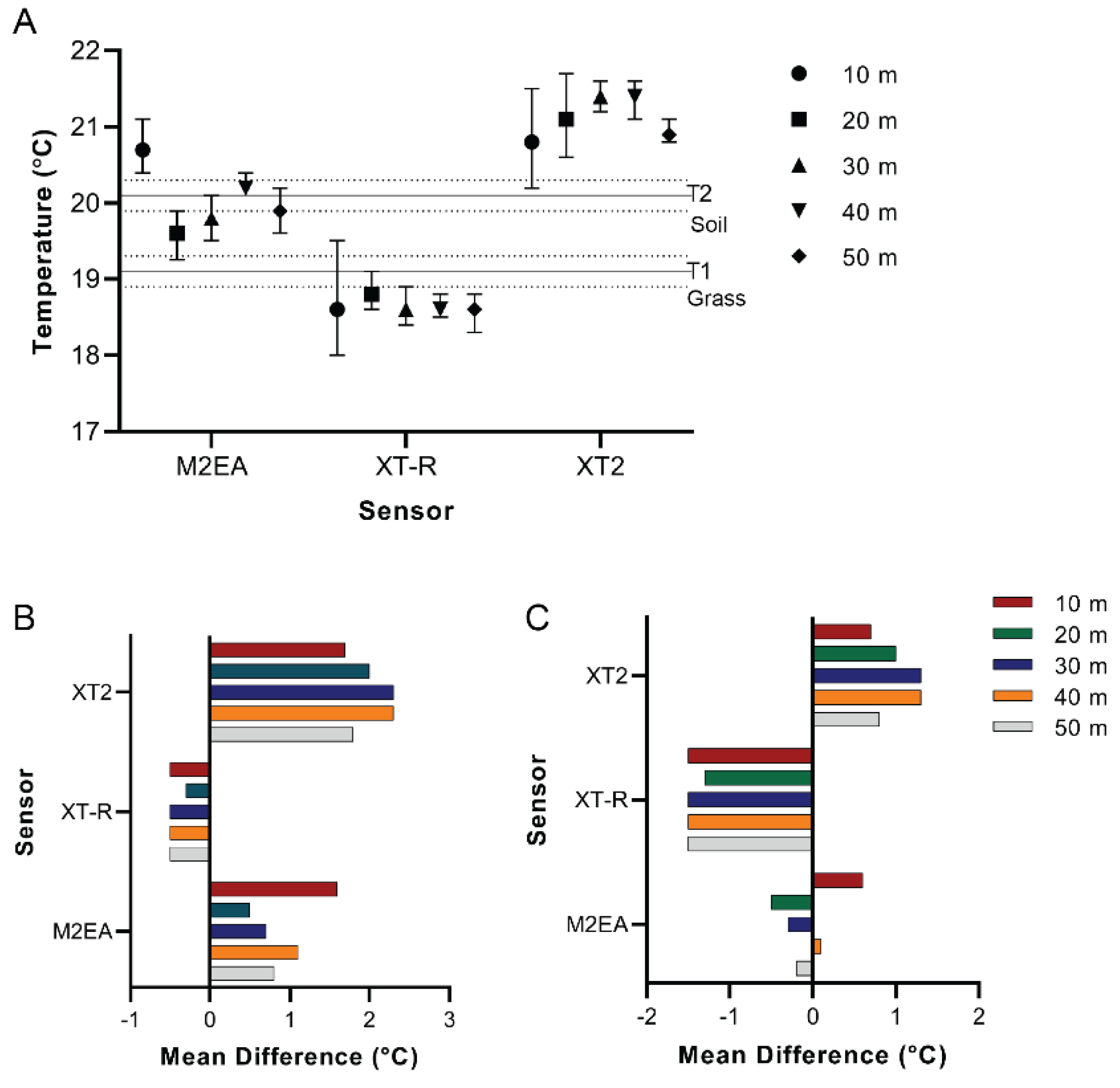
Results for vegetation was obtained by comparing the TIRI data from each camera at each height with that of the in situ ground measurements are shown in Figure 15 and Figure 16. For the most part, the grass temperature estimate from the M2EA lies between the in situ temperatures obtained for grass canopy and soil for both T1/T2 (Figure 15) and T3/T4 locations (Figure 16). The actual location (on the temperatures axis) that the grass and the image measurements lies at is a function of air temperature, air space within the canopy and the coverage of the vegetation over the soil. As the soil sensor was emplaced 5 cm below the surface, and below the root mat, its value represents the true temperature of the upper surface of the soil. As seen in Figure 13, the TIRI temperature values from the M2EA camera, exhibit the greatest deviation from the in situ measurements. As with the concrete example in Figure 13, the source of this anomaly has yet to be determined. At both vegetation sites, across heights, the XT-R camera is most similar to the measurements of the in situ soil probes (0.3–0.8 °C difference). In contrast, the XT2 is most similar to the grass canopy in situ probes at both vegetation sites (0.7–1.3 °C difference) (Figure 15 and Figure 16). As expected, for all three cameras, the greatest variability in the temperature of the grass pixels is seen at the 10 m height (smallest pixels). For the XT-R and XT2, the range of grass pixel values is lowest but similar across the 30–50 m heights. As seen with the concrete target (Figure 13), the deviation of the TIRI estimated temperatures is mostly greater than the bias determined from the blackbody experiment (Table 3); nevertheless, the differences seen for the grass canopies and soil are small for all sensors (<2.5 °C and <2.0 °C respectively).
4. Discussion
The overall results obtained from the blackbody work, show that each camera has performed within the uncertainty envelopes of their calibration, and thus, are validated for use within the constraints of that calibration. Further, this work has shown that there is essentially, no appreciable difference in validation results or camera performance as a function of distance—under the constraints of 2 m and 4 m distances—which may be extended with caution to suggest that these same results hold when the distance is doubled if the source is relatively close to the camera. All three cameras showed high linearity in their response and low errors for all targets (blackbody, concrete, soil) with differences <2 °C between them (except for the blackbody measurements with the XT-R camera at 5 °C and 40 °C—which are outside of the environmental range of the field study).
It is evident from the results of the concrete targets and both vegetation sites, that temperatures retrieved with the XT-R camera are consistently lower than those of the other two cameras. While the temperature retrievals for the vegetation and soil plots show that the XT2 overestimates the grass temperature they also show that the M2EA falls between the values for the vegetation and the soil. However, all the systems generally performed within 2 °C (i.e., ΔT ≤ 2 °C) of the in situ measured temperatures of the targets.
In the context of how this work fits into that of previous studies, our methodology and results have taken several parameters into account that were either missing or were identified as topics of further work. For example, the process we showed herein is very different from [36], due primarily to our night time operations at the field site; further, we also consider environmental factors, such as air temperature and humidity. In [36], the in-field blackbody target was imaged; however, no accounting for environmental factors such as wind, humidity or air temperature was performed but rather considered as a portion of a common residual bias offset of 2.67 °C. Furthermore, the work was performed during the daytime (between 07:10 and 14:00) when solar heating effects have a significant non-linear impact [54,66,67] even over the timespan of an RPAS flight—typically under 30 min.
Comparing our current work to that in [37], shows the similarities in thought behind the use of the indoor blackbody to characterize the sensor before flight campaigns. While [37] provides a vicarious calibration, we have focused on validation for the reasons outlined previously in this work (calibration requires a highly controlled environment and exceedingly accurate radiometric instrumentation—as was the outcome concluded in [37]). Further, in [37], there was no mention of collecting or addressing environmental data nor the use of any in-field thermal calibration targets, although they did validate their neural network-based photogrammetry process which aided in improving the accuracy of their imaging. Also, as in [36], [37] collected their field-based TIRI during the daytime and therefore, previous statements for [36] on that practice also apply to the work of [37].
In the work by [38], a constant 0 °C value for the imaged surface of melting snow targets was used; however, it was identified that the vicarious calibration method employed, performed better without the natural target of the melting snow surface. The melting snow target temperature was found to be variable and correlated to underlying forest vegetation conditions. Moreover, retrieved TIRI data showed spatial pixel size temperature dependencies, angular dependencies as well as mixed pixel issues with more dense forest canopy. In our work, we have developed a method that is not being influenced by such sources.
The calibration work of [39] produced TIRI of an ice bath for evaluation. While [39] provides support for the idea of requiring accurate RPAS TIRI, it has not provided those results in a field environment under RPAS flight conditions—which is stated within [39] as a suggestion for further work. The work of this study has developed a field-level validation method (not the same as calibration) in order to determine if the calibration (be it manufacturer or based on [39], or similar methods) remains applicable near the time of the RPAS work.
In our study, all cameras have performed as per specifications, and therefore, it may be difficult to decide which of these cameras to use. As all three produce essentially identical ground pixel sizes (the M2EA produces slightly larger pixels, due to the slightly larger FOV, ~0–2 mm difference within an image square pixel of ~10 cm side length, and have nearly the same noise floors (<50 mK), the decision may be best decided by the non-thermal portions of the system. Both the M300 airframe and XT2 camera have ratings of IP45 and IP 44, respectively, and are thus, essentially waterproof—neither of the other two cameras, nor airframes, have an IP rating. The XT-R camera requires a stationary drone to take the images (otherwise the results have considerable blur), while the XT2 and M2EA can acquire with slow but continuous flight speeds. The M2EA is, by far, the easiest to transport, followed by the M300 and finally the M600P, which is difficult due to the 67 cm length of side and cube shaped case. While the M300 and M600P require a separate ground station with tripod to function in RTK mode, the M2EA is fully self-contained and only requires a Wi-Fi connection and incoming corrections for RTK mode. The inclusion of a 4K visible RGB camera coincident with the thermal cameras with the M2EA and XT2 is a large advantage in many applications during daytime hours. However, care must be taken with all three cameras not to burn the thermal sensor from incoming solar radiation. For applications that require stealth, such as wildlife studies [9,11], RPAS size and rotor noise (more significant with the M600P) is a primary concern. Further, payload and ancillary sensors (hyperspectral, LiDAR, etc) are often a complementary desire with TIRI, therefore RPAS payload capability will play a dominant part of the selection criteria. Finally, one other non-technical consideration that has a tremendous impact on operations is that the XT-R camera has an Export Control Classification Number (6A003.b.4.b., [46]) and is therefore, very difficult to travel across international borders.
While it is also important to note that the XT-R and XT2 are no longer manufactured, they, continue to be very much in use [9,11,13,17,18,21,22,23,24,26,27,28,68,69] and are sure to be primary instruments in new works to come. The M2EA is relatively new and highly capable, being able to compete (results-wise) with the XT2 system.
Finally, although this work has been applied to TIRI in the LWIR region, it has been derived in accordance with basic properties and principles of the TIR region of the electromagnetic spectrum. As a result, we suggest that it is also applicable to the Mid-Wave InfraRed (3–7.5 μm) region and, therefore, it can be used with all TIRI data from within the TIR.
5. Conclusions
In this work, we have developed a new TIRI validation methodology that has been applied to LWIR imagery (7.5 μm to 14 μm) taken of a blackbody source (indoors) and to real-world field conditions (outdoor) using instrumented concrete and vegetation sites as validation targets. We have tested our method on three popular LWIR TIRI cameras (the Zenmuse XT-R, Zenmuse XT2 and the M2EA) that are operated by three different popular DJI RPAS platforms—the Matrice 600 Pro, the M300 RTK and the Mavic 2 Enterprise Advanced. Results of the blackbody work over the temperatures expected in the field site show a highly linearized response for each sensor as well as a small temperature bias. All TIRI camera measurements were validated (by surface thermal sensors) to be within the stated tolerances of uncertainty for the cameras. Environmental parameters (air temperature, humidity, pressure and wind) were measured for several hours before TIRI data was collected. Wind cooling was not a factor up to 2 h prior to data collection. In-field TIRI results from 10 m to 50 m heights, images show absolute temperature retrievals of the target materials (concrete and two vegetation sites) that were within the specifications of the cameras. The methodology has been developed under the condition that it should be applicable to RPAS operators who need to verify their equipment either pre or post operations.
Author Contributions
Conceptualization, G.L. and M.K.; methodology, G.L., M.K., J.P.A.-M., O.L. and A.T.; software, M.K. and J.P.A.-M.; validation, M.K., O.L. and G.L.; formal analysis, G.L. and M.K.; investigation, G.L., M.K., J.P.A.-M. and O.L.; resources, G.L., M.K. and O.L.; data curation, M.K. and J.P.A.-M.; writing—original draft preparation, G.L., M.K.; writing—review and editing, G.L., M.K., J.P.A.-M., A.T. and O.L. All authors have read and agreed to the published version of the manuscript.
Funding
This research received external funding by the Natural Sciences and Engineering Research Council Canada (NSERC), Discovery Grant program to M.K.
Data Availability Statement
Data available upon request to the corresponding author.
Acknowledgments
We would like to thank Stephen Scheunert for use of the RPAS field site, Paul Mondor for support at the field site and, Calvin Leblanc for support with the blackbody work. We also thank Iryna Borshchova, Greg Craig and two anonymous reviewers for their input that helped to improve the manuscript. Finally, we would like to thank Tim Mammatt from Aethea for use of the ThermoConverter software and information about the M2EA, and Kevin Toderel from RMUS for help with the M2EA.
Conflicts of Interest
The authors declare no conflict of interest.
Appendix A

Table A1.
Summary data from the blackbody measurements.
| Camera | Distance (m) | Mean Blackbody Temp. (+/−0.4 °C) | Mean Measured Temp. (°C) | Stdev. (°C) |
|---|---|---|---|---|
| M2EA | 2 | 5 | 1.87 | 0.13 |
| M2EA | 2 | 10 | 7.77 | 0.12 |
| M2EA | 2 | 15 | 13.57 | 0.11 |
| M2EA | 2 | 20 | 19.10 | 0.10 |
| M2EA | 2 | 25 | 24.37 | 0.11 |
| M2EA | 2 | 30 | 30.03 | 0.10 |
| M2EA | 2 | 35 | 35.63 | 0.11 |
| M2EA | 2 | 40 | 41.20 | 0.10 |
| M2EA | 4 | 5 | 3.70 | 0.16 |
| M2EA | 4 | 10 | 8.90 | 0.15 |
| M2EA | 4 | 15 | 13.77 | 0.10 |
| M2EA | 4 | 20 | 18.35 | 0.10 |
| M2EA | 4 | 25 | 24.40 | 0.11 |
| M2EA | 4 | 30 | 29.80 | 0.12 |
| M2EA | 4 | 35 | 34.77 | 0.13 |
| M2EA | 4 | 40 | 39.97 | 0.13 |
| XT-R | 2 | 5 | 3.23 | 0.11 |
| XT-R | 2 | 10 | 9.83 | 0.09 |
| XT-R | 2 | 15 | 13.27 | 0.09 |
| XT-R | 2 | 20 | 18.93 | 0.07 |
| XT-R | 2 | 25 | 23.33 | 0.08 |
| XT-R | 2 | 30 | 30.53 | 0.07 |
| XT-R | 2 | 35 | 33.20 | 0.09 |
| XT-R | 2 | 40 | 39.60 | 0.08 |
| XT-R | 4 | 5 | 3.13 | 0.10 |
| XT-R | 4 | 10 | 8.97 | 0.10 |
| XT-R | 4 | 15 | 15.43 | 0.07 |
| XT-R | 4 | 20 | 18.17 | 0.08 |
| XT-R | 4 | 25 | 23.80 | 0.06 |
| XT-R | 4 | 30 | 30.00 | 0.06 |
| XT-R | 4 | 35 | 34.13 | 0.07 |
| XT-R | 4 | 40 | 37.13 | 0.08 |
| XT2 | 2 | 5 | 4.23 | 0.11 |
| XT2 | 2 | 10 | 8.87 | 0.10 |
| XT2 | 2 | 15 | 14.80 | 0.09 |
| XT2 | 2 | 20 | 20.57 | 0.10 |
| XT2 | 2 | 25 | 25.43 | 0.08 |
| XT2 | 2 | 30 | 29.17 | 0.08 |
| XT2 | 2 | 35 | 35.43 | 0.08 |
| XT2 | 2 | 40 | 39.80 | 0.08 |
| XT2 | 4 | 5 | 4.23 | 0.12 |
| XT2 | 4 | 10 | 9.03 | 0.10 |
| XT2 | 4 | 15 | 14.90 | 0.10 |
| XT2 | 4 | 20 | 19.90 | 0.08 |
| XT2 | 4 | 25 | 25.07 | 0.09 |
| XT2 | 4 | 30 | 30.43 | 0.09 |
| XT2 | 4 | 35 | 34.57 | 0.08 |
| XT2 | 4 | 40 | 40.07 | 0.10 |
References
- Stanković, M.; Mirza, M.M.; Karabiyik, U. UAV Forensics: DJI Mini 2 Case Study. Drones 2021, 5, 49. [Google Scholar] [CrossRef]
- Burgués, J.; Marco, S. Environmental chemical sensing using small drones: A review. Sci. Total Environ. 2020, 748, 141172. [Google Scholar] [CrossRef]
- Lakshman, S.A.; Ebenezer, D. Ebenezer, Integration of internet of things and drones and its future applications. Mater. Today Proc. 2021, 47, 944–949. [Google Scholar] [CrossRef]
- Shahmoradi, J.; Talebi, E.; Roghanchi, P.; Hassanalian, M. A Comprehensive Review of Applications of Drone Technology in the Mining Industry. Drones 2020, 4, 34. [Google Scholar] [CrossRef]
- Witczuk, J.; Pagacz, S.; Zmarz, A.; Cypel, M. Exploring the feasibility of unmanned aerial vehicles and thermal imaging for ungulate surveys in forests—Preliminary results. Int. J. Remote Sens. 2018, 39, 5504–5521. [Google Scholar] [CrossRef]
- Ellsäßer, F.; Röll, A.; Ahongshangbam, J.; Waite, P.-A.; Schuldt, B.; Hölscher, D. Predicting Tree Sap Flux and Stomatal Conductance from Drone-Recorded Surface Temperatures in a Mixed Agroforestry System—A Machine Learning Approach. Remote Sens. 2020, 12, 4070. [Google Scholar] [CrossRef]
- Alekseychik, P.; Katul, G.; Korpela, I.; Launiainen, S. Eddies in motion: Visualizing boundary-layer turbulence above an open boreal peatland using UAS thermal videos. Atmos. Meas. Tech. 2021, 14, 3501–3521. [Google Scholar] [CrossRef]
- Hyun, C.-U.; Park, M.; Lee, W.Y. Remotely Piloted Aircraft System (RPAS)-Based Wildlife Detection: A Review and Case Studies in Maritime Antarctica. Animals 2020, 10, 2387. [Google Scholar] [CrossRef]
- Ireland, A.W.; Palandro, D.A.; Garas, V.Y.; Woods, R.W.; Davi, R.A.; Butler, J.D.; Gibbens, D.M.; Gibbens, J.S., Jr. Testing unmanned aerial systems for monitoring wildlife at night. Wildl. Soc. Bull. 2019, 43, 182–190. [Google Scholar] [CrossRef] [Green Version]
- Beaver, J.T.; Baldwin, R.W.; Messinger, M.; Newbolt, C.H.; Ditchkoff, S.S.; Silman, M.R. Evaluating the Use of Drones Equipped with Thermal Sensors as an Effective Method for Estimating Wildlife. Wildl. Soc. Bull. 2020, 44, 434–443. [Google Scholar] [CrossRef]
- Scholten, C.N.; Kamphuis, A.J.; Vredevoogd, K.J.; Lee-Strydhorst, K.G.; Atma, J.L.; Shea, C.B.; Lamberg, O.N.; Proppe, D.S. Real-time thermal imagery from an unmanned aerial vehicle can locate ground nests of a grassland songbird at rates similar to traditional methods. Biol. Conserv. 2019, 233, 241–246. [Google Scholar] [CrossRef]
- Melis, M.T.; Da Pelo, S.; Erbì, I.; Loche, M.; Deiana, G.; Demurtas, V.; Meloni, M.A.; Dessì, F.; Funedda, A.; Scaioni, M.; et al. Thermal Remote Sensing from UAVs: A Review on Methods in Coastal Cliffs Prone to Landslides. Remote Sens. 2020, 12, 1971. [Google Scholar] [CrossRef]
- Zhang, R.; Li, H.; Duan, K.; You, S.; Liu, K.; Wang, F.; Hu, Y. Automatic Detection of Earthquake-Damaged Buildings by Integrating UAV Oblique Photography and Infrared Thermal Imaging. Remote Sens. 2020, 12, 2621. [Google Scholar] [CrossRef]
- Marotta, E.; Peluso, R.; Avino, R.; Belviso, P.; Caliro, S.; Carandente, A.; Chiodini, G.; Macedonio, G.; Avvisati, G.; Marfè, B. Thermal Energy Release Measurement with Thermal Camera: The Case of La Solfatara Volcano (Italy). Remote Sens. 2019, 11, 167. [Google Scholar] [CrossRef] [Green Version]
- Gaitani, N.; Burud, I.; Thiis, T.; Santamouris, M. High-resolution spectral mapping of urban thermal properties with Unmanned Aerial Vehicles. Build. Environ. 2017, 121, 215–224. [Google Scholar] [CrossRef]
- Naughton, J.; McDonald, W. Evaluating the Variability of Urban Land Surface Temperatures Using Drone Observations. Remote Sens. 2019, 11, 1722. [Google Scholar] [CrossRef] [Green Version]
- Bayomi, N.; Nagpal, S.; Rakha, T.; Fernandez, J.E. Building envelope modeling calibration using aerial thermography. Energy Build. 2021, 233, 110648. [Google Scholar] [CrossRef]
- Park, S.-I.; Ryu, T.-H.; Choi, I.-C.; Um, J.-S. Evaluating the Operational Potential of LRV Signatures Derived from UAV Imagery in Performance Evaluation of Cool Roofs. Energies 2019, 12, 2787. [Google Scholar] [CrossRef] [Green Version]
- Hill, A.C.; Laugier, E.J.; Casana, J. Archaeological Remote Sensing Using Multi-Temporal, Drone-Acquired Thermal and Near Infrared (NIR) Imagery: A Case Study at the Enfield Shaker Village, New Hampshire. Remote Sens. 2020, 12, 690. [Google Scholar] [CrossRef] [Green Version]
- DiNapoli, R.J.; Lipo, C.P.; de Smet, T.S.; Hunt, T.L. Thermal Imaging Shows Submarine Groundwater Discharge Plumes Associated with Ancient Settlements on Rapa Nui (Easter Island, Chile). Remote Sens. 2021, 13, 2531. [Google Scholar] [CrossRef]
- Adamopoulos, E.; Rinaudo, F. UAS-Based Archaeological Remote Sensing: Review, Meta-Analysis and State-of-the-Art. Drones 2020, 4, 46. [Google Scholar] [CrossRef]
- Turner, R.M.; MacLaughlin, M.M.; Iverson, S.R. Identifying and mapping potentially adverse discontinuitie in underground excavations using thermal and multispectral UAV imagery. Eng. Geol. 2020, 266, 105470. [Google Scholar] [CrossRef]
- He, X.; Yang, X.; Luo, Z.; Guan, T. Application of unmanned aerial vehicle (UAV) thermal infrared remote sensing to identify coal fires in the Huojitu coal mine in Shenmu city, China. Sci. Rep. 2020, 10, 13895. [Google Scholar] [CrossRef] [PubMed]
- Zhao, Y.; Sun, B.; Liu, S.; Zhang, C.; He, X.; Xu, D.; Tang, W. Identification of mining induced ground fissures using UAV and infrared thermal imager: Temperature variation and fissure evolution. ISPRS J. Photogramm. Remote Sens. 2021, 180, 45–64. [Google Scholar] [CrossRef]
- Zheng, H.; Zhong, X.; Yan, J.; Zhao, L.; Wang, X. A Thermal Performance Detection Method for Building Envelope Based on 3D Model Generated by UAV Thermal Imagery. Energies 2020, 13, 6677. [Google Scholar] [CrossRef]
- Rakha, T.; Gorodetsky, A. Review of Unmanned Aerial System (UAS) applications in the built environment: Towards automated building inspection procedures using drones. Autom. Constr. 2018, 93, 252–264. [Google Scholar] [CrossRef]
- Leggiero, M.; Andrew, B.; Elliott, R.; Indergaard, J.; Sharma, J.B.; Vogel, T. Radiative heat loss estimation of building envelopes based on 3D thermographic models utilizing small unmanned aerial systems (sUAS). Energy Build. 2021, 244, 110957. [Google Scholar] [CrossRef]
- Deane, S.; Avdelidis, N.P.; Ibarra-Castanedo, C.; Zhang, H.; Nezhad, H.Y.; Williamson, A.A.; Mackley, T.; Maldague, X.; Tsourdos, A.; Nooralishahi, P. Comparison of Cooled and Uncooled IR Sensors by Means of Signal-to-Noise Ratio for NDT Diagnostics of Aerospace Grade Composites. Sensors 2020, 20, 3381. [Google Scholar] [CrossRef]
- Crastes, A., Sr.; Ruiter, M.; Gierkink, S., Sr.; Brunelle, J., Sr. Recent uncooled IR development based on state of the art digital ROIC. Infrared Sensors, Devices, and Applications XI. Int. Soc. Opt. Photonics 2021, 8, 118310H. [Google Scholar] [CrossRef]
- Tankut, F.; Cologlu, M.H.; Askar, H.; Ozturk, H.; Dumanli, H.K.; Oruc, F.; Tilkioglu, B.; Ugur, B.; Akar, O.S.; Tepegoz, M.; et al. An 80 × 80 microbolometer type thermal imaging sensor using the LWIR-band CMOS infrared (CIR) technology. Infrared Technology and Applications XLIII. Int. Soc. Opt. Photonics 2017, 10177, 101771X. [Google Scholar] [CrossRef]
- Laurent, L.; Yon, J.-J.; Moulet, J.-S.; Roukes, M.; Duraffourg, L. 12-µm-Pitch Electromechanical Resonator for Thermal Sensing. Phys. Rev. Appl. 2018, 9, 024016. [Google Scholar] [CrossRef] [Green Version]
- Kennedy, H.V. Modeling noise in thermal imaging systems. Infrared Imaging Systems: Design, Analysis, Modeling, and Testing IV. Int. Soc. Opt. Photonics 1993, 1969, 66–77. [Google Scholar] [CrossRef]
- Sharma, P.; Dell, J.; Parish, G.; Keating, A. Engineering 1/f noise in porous silicon thin films for thermal sensing applications. Microporous Mesoporous Mater. 2021, 324, 111302. [Google Scholar] [CrossRef]
- Yu, L.; Guo, Y.; Zhu, H.; Luo, M.; Han, P.; Ji, X. Low-Cost Microbolometer Type Infrared Detectors. Micromachines 2020, 11, 800. [Google Scholar] [CrossRef]
- Holst, G.C. Common Sense Approach to Thermal Imaging; SPIE Optical Engineering Press: Washington, DC, USA, 2000. [Google Scholar]
- Torres-Rua, A. Vicarious calibration of suas microbolometer temperature imagery for estimation of radiometric land surface temperature. Sensors 2017, 17, 1499. [Google Scholar] [CrossRef] [PubMed] [Green Version]
- Ribeiro-Gomes, K.; Hernández-López, D.; Ortega, J.F.; Ballesteros, R.; Poblete, T.; Moreno, M.A. Uncooled Thermal Camera Calibration and Optimization of the Photogrammetry Process for UAV Applications in Agriculture. Sensors 2017, 17, 2173. [Google Scholar] [CrossRef]
- Pestana, S.; Chickadel, C.C.; Harpold, A.; Kostadinov, T.S.; Pai, H.; Tyler, S.; Webster, C.; Lundquist, J.D. Bias correction of airborne thermal infrared observations over forests using melting snow. Water Resour. Res. 2019, 55, 11331–11343. [Google Scholar] [CrossRef]
- Aragon, B.; Johansen, K.; Parkes, S.; Malbeteau, Y.; Al-Mashharawi, S.; Al-Amoudi, T.; Andrade, C.F.; Turner, D.; Lucieer, A.; McCabe, M.F. A Calibration Procedure for Field and UAV-Based Uncooled Thermal Infrared Instruments. Sensors 2020, 20, 3316. [Google Scholar] [CrossRef] [PubMed]
- Drone Industry Insights. Top 10 Drone Manufacturers’ Market Shares in the US; Drone Industry Insights UG: Hamburg, Germany, 2019. [Google Scholar]
- DJI Science and Technology Co., Ltd. Mavic 2 Enterprise Advanced User Manual v 1.0. 03, Shenzhen, China. 2021. Available online: https://dl.djicdn.com/downloads/Mavic_2_Enterprise_Advanced/20210331/Mavic_2_Enterprise_Advanced_User_Manual_EN.pdf (accessed on 13 October 2021).
- DJI Science and Technology Co., Ltd. Matrice 600 Pro User Manual V1.0. Shenzhen, China. 2018. Available online: https://dl.djicdn.com/downloads/m600%20pro/1208EN/Matrice_600_Pro_User_Manual_v1.0_EN_1208.pdf (accessed on 13 October 2021).
- DJI Science and Technology Co., Ltd. Matrice 300 RTK User Manual V1.8. Shenzhen, China. 2021. Available online: https://dl.djicdn.com/downloads/matrice-300/20210419UM/M300_RTK_User_Manual_EN_v1.8_20210419.pdf (accessed on 13 October 2021).
- Kalacska, M.; Lucanus, O.; Arroyo-Mora, J.P.; Laliberté, É.; Elmer, K.; Leblanc, G.; Groves, A. Accuracy of 3D Landscape Reconstruction without Ground Control Points Using Different UAS Platforms. Drones 2020, 4, 13. [Google Scholar] [CrossRef] [Green Version]
- DJI Science and Technology Co., Ltd. Zenmuse XT2 Thermal by FLIR User Manual v1.0, 04, Shenzhen, China. 2018. Available online: https://dl.djicdn.com/downloads/Zenmuse%20XT%202/Zenmuse_XT_2_User_Manual_v1.0_en_.pdf (accessed on 13 October 2021).
- DJI Science and Technology Co., Ltd. Zenmuse XT Powered by FLIR User Manual v1.2, 05, Shenzhen, China. 2016. Available online: https://dl.djicdn.com/downloads/zenmuse_xt/en/Zenmuse_XT_User_Manual_V1.2_en_0708.pdf (accessed on 13 October 2021).
- Tiesinga, E.; Mohr, P.J.; Newell, D.B.; Taylor, B.N. CODATA recommended values of the fundamental physical constants: 2018. Rev. Mod. Phys. 2021, 93, 025010. [Google Scholar] [CrossRef]
- Minkina, W.; Dudzik, S. Infrared Thermography: Erros and Uncertainties; John Wiley & Sons: Hoboken, NJ, USA, 2009. [Google Scholar]
- Garcia-Santos, V.; Valor, E.; Caselles, V.; Mira, M.; Galve, J.M.; Coll, C. Evaluation of Different Methods to Retrieve the Hemispherical Downwelling Irradiance in the Thermal Infrared Region for Field Measurements. IEEE Trans. Geosci. Rem. Sens. 2013, 51, 4. [Google Scholar] [CrossRef]
- Fluke Corporation. Fluke Calibration 4180, 4181 Precision Infrared Calibrator. Operators Manual. November 2020. Available online: https://us.flukecal.com/products/process-calibration-tools/temperature-calibrators/infrared-calibrators/4180-4181-precision-?quicktabs_product_details=4 (accessed on 13 October 2021).
- da Cunha, A.R. Evaluation of measurement errors of temperature and relative humidity from HOBO data logger under different conditions of exposure to solar radiation. Envron. Monit. Assess. 2015, 187, 236. [Google Scholar] [CrossRef]
- Abdullahi, M.G.; Husini, E.M.; Ibrahim, A.O.; Collins, K.; Arabi, O.F.; Bashir, F.M. Architectural Experimental Field Measurement Process and Procedure using Case Study. Solid State Technol. 2021, 64, 2. [Google Scholar]
- Shawesh, R.; Mohamed, M. Post-occupancy evaluation of outdoor thermal comfort in hot arid zone. Int. J. Low Carb. Technol. 2020, 16, 1. [Google Scholar] [CrossRef]
- Lozano-Parra, J.; Pulido, M.; Lozano-Fondón, C.; Schnabel, S. How do Soil Moisture and Vegetation Covers Influence Soil Temperature in Drylands of Mediterranean Regions? Water 2018, 10, 1747. [Google Scholar] [CrossRef] [Green Version]
- Cengal, Y.A. Heat Transfer: A Practical Approach, 2nd ed.; McGraw–Hill: New York, NY, USA, 2002. [Google Scholar]
- Balaras, C.A.; Argiriou, A.A. Infrared thermography for building diagnostics. Energy Build. 2002, 34, 2. [Google Scholar] [CrossRef]
- Lehmann, B.; Wakili, K.G.; Frank, T.; Collado, B.V.; Tanner, C. Effects of individual climatic parameters on the infrared thermography of buildings. Appl. Energy 2013, 110, 29–43. [Google Scholar] [CrossRef]
- Jonsson, B.; Zinko, H. Quantitative Heat Loss Analysis of Heat- and Coolant Distribution Pipes by Means of Thermography; NOVEM: Vorbach, Germany, 1993; ISBN 90-72130-95-2. [Google Scholar]
- FluxTeq LLC. PHFS-01e Heat Flux Sensor Datasheet. Available online: https://d7c61e62-ec2b-486f-b3c3-d005ddd2f7d8.filesusr.com/ugd/b0a63e_e2f8d1846d244ead8946fe3d870ce7e2.pdf (accessed on 13 October 2021).
- Davies, J.A.; Idso, S.B. Estimating the Surface Radiation Balance and Its Components. Modification of the Aerial Environment of Plants. ASAE Monograph; American Society of Agricultural: St. Joseph, MI, USA, 1979; pp. 183–210. [Google Scholar]
- Tu, L.; Qin, Z.; Yang, L.; Wang, F.; Geng, J.; Zhao, S. Identifying the Lambertian Property of Ground Surfaces in the Thermal Infrared Region via Field Experiments. Remote Sens. 2017, 9, 481. [Google Scholar] [CrossRef] [Green Version]
- Humes, K.S.; Kustas, W.P.; Moran, M.S.; Nichols, W.D.; Weltz, M.A. Variability of emissivity and surface temperature over a sparsely vegetated surface. Water Resour. Res. 1994, 30, 1299–1310. [Google Scholar] [CrossRef]
- Kotthaus, S.; Smith, T.E.L.; Wooster, M.J.; Grimmond, C.S.B. Derivation of an urban materials spectral library through emittance and reflectance spectroscopy. ISPRS J. Photogramm. Remote Sens. 2014, 94, 194–212. [Google Scholar] [CrossRef] [Green Version]
- Sagan, V.; Maimaitijiang, M.; Sidike, P.; Eblimit, K.; Peterson, K.T.; Hartling, S.; Esposito, F.; Khanal, K.; Newcomb, M.; Pauli, D.; et al. UAV-Based High Resolution Thermal Imaging for Vegetation Monitoring, and Plant Phenotyping Using ICI 8640 P, FLIR Vue Pro R 640, and thermoMap Cameras. Remote Sens. 2019, 11, 330. [Google Scholar] [CrossRef] [Green Version]
- Hackl, H.; Baresel, J.P.; Mistele, B.; Hu, Y.; Schmidhalter, U. A Comparison of Plant Temperatures as Measured by Thermal Imaging and Infrared Thermometry. J. Agron. Crop Sci. 2012, 198, 415–429. [Google Scholar] [CrossRef] [Green Version]
- Brevik, E.C.; Fenton, T.E.; Horton, R. Effect of Daily Soil Temperature Fluctuations on Soil Electrical Conductivity as Measured with the Geonics® EM-38. Precis. Agric. 2004, 5, 145–152. [Google Scholar] [CrossRef]
- Singh, R.K.; Sharma, R.V. Numerical analysis for ground temperature variation. Geotherm. Energy 2017, 5, 22. [Google Scholar] [CrossRef] [Green Version]
- Patrucco, G.; Cortese, G.; Tonolo, F.G.; Spanò, A. Thermal and optical data fusion supporting built heritage analyses. Int. Arch. Photogramm. Remote Sens. Spat. Inf. Sci. 2020, 43, 619–626. [Google Scholar] [CrossRef]
- Kuczyńska, A.; Jarnuszewski, G.; Nowakowska, M.; Wexler, S.K.; Wiśniowski, Z.; Burczyk, P.; Durkowski, T.; Woźnicka, M. Identifying causes of poor water quality in a Polish agricultural catchment for designing effective and targeted mitigation measures. Sci. Total Environ. 2021, 765, 144125. [Google Scholar] [CrossRef]
Figure 1.
RPAS systems and cameras in this study. (A) The M600P (left), M2EA (center) and M300 (right). (B) the Zenmuse XT-R with gimbal, (C) the M2EA form-integrated thermal (upper) and visible (lower) cameras and, (D) the Zenmuse XT2 thermal (right) and visible (left) cameras. The cameras are shown in the same order from L-R as the airframes with which they are compatible.

Figure 2.
Illustration of the various sources of thermal infrared radiation to be considered with RPAS estimations of surface temperature in absence of nearby objects which would radiate energy into the scene. The arrows are representative of the relative contribution of each source. Three materials (grass, concrete, InfraGold) with a range of emissivity values considered in this study are shown. Atmospheric transmission decreases with increased distance between the TIRI sensor and the target. Atmospheric constituents such as water, smoke, dust, etc. all influence thermal transmission, with increasing significance at greater distances and/or as the concentration of the constituents increases.

Figure 3.
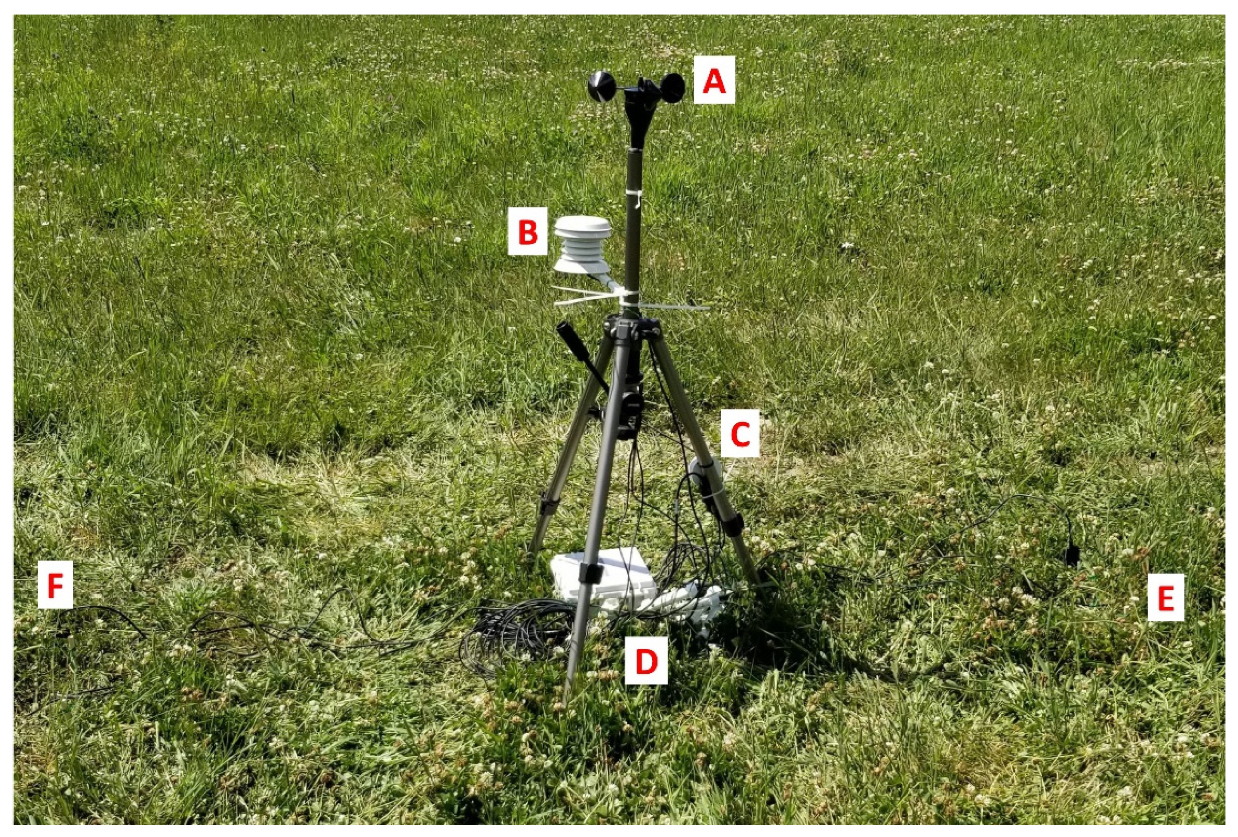
Validation set-up that would be typical of a workspace pre/post RPAS operations. The tripod (A) that carries the environmental sensors for air temperature, RH, pressure and air movement, the FLUKE 4180 blackbody (B) and the M600P airframe with the XT-R camera (C).
Figure 3.
Validation set-up that would be typical of a workspace pre/post RPAS operations. The tripod (A) that carries the environmental sensors for air temperature, RH, pressure and air movement, the FLUKE 4180 blackbody (B) and the M600P airframe with the XT-R camera (C).

Figure 4.
Field site near Vaudreuil-Dorion, QC (top panel) with the light blue/green box representing the area of the investigation and the instrumented ground site location. Ground site set-up (lower panels) including: differentialRTK base station for the M300 (A), and for the M600P (B), environmental monitoring station and vegetation validation site (C), the InfraGold dark sky diffuse reflectance panel (D) with foil protection covering that was removed before data collection, and the concrete slab target (E) with three thermal flux sensors (used for deriving temperature) indicated by the red arrow in the lower left panel. Photographs were taken during the day for clarity. The orange circular feature in the lower left panel (with an “H”) shows the launch area for the RPAS vehicles.

Figure 5.
Environmental monitoring station and vegetation target from Figure 4. The photograph shows the emplacement of the anemometer (A) at 1.0 m height, the Tair and RH (one unit) under a solar radiative shield (B), air pressure (C) and, control electronics and data collection units (D). Also shown are the vegetation/soil target areas of T1/T2 (E) and T3/T4 (F) at 1.0 m distance from the center of the tripod location. Soil temperature probes (T2 and T4) were implanted at a depth of 5 cm directly below the in-canopy temperature sensors (T1 and T3).

Figure 6.
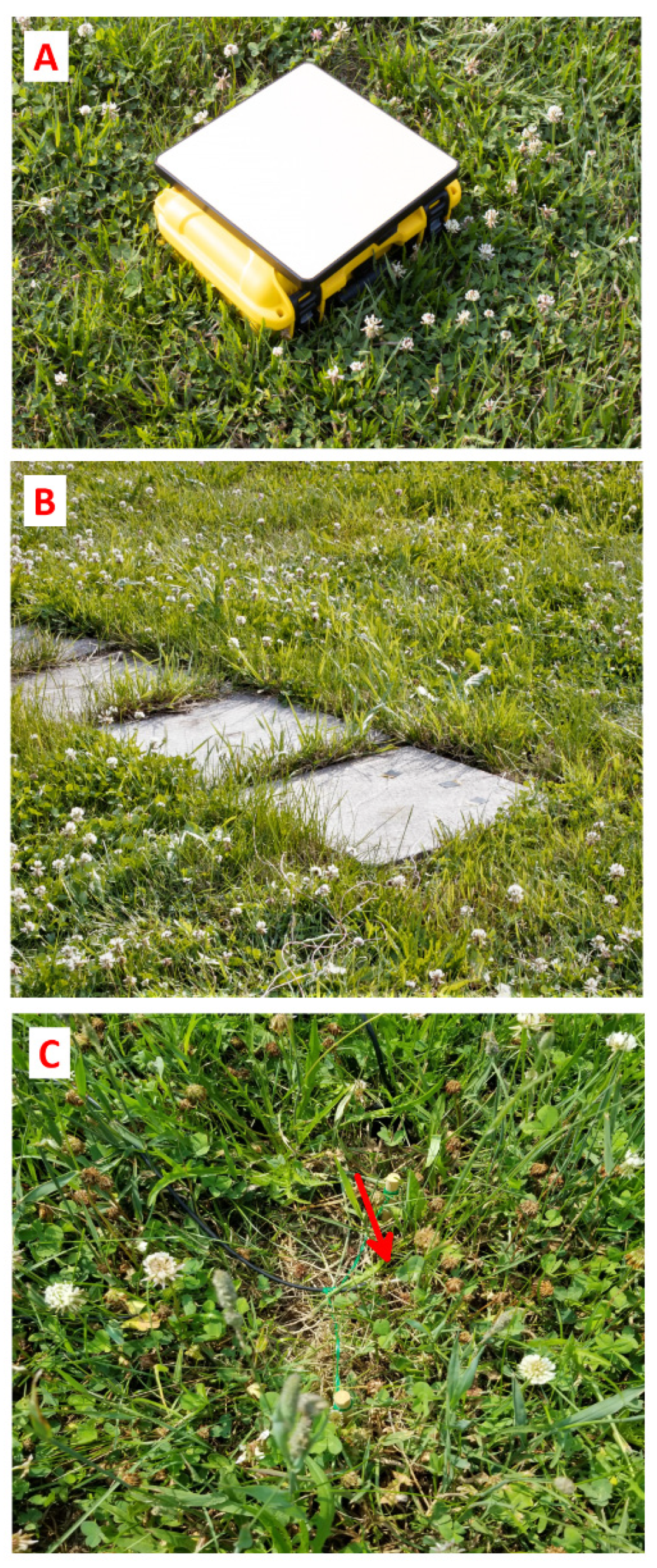
Target materials used for comparison. (A) InfraGold panel atop a plastic storage box, used as a platform to keep the surface debris free. (B) Concrete patio stones with three heat flux sensors (black squares on the concrete slab—as also indicated in Figure 4 label E) from which temperature was derived. The left-most sensor did not stay adhered to the surface and therefore, the data were not used. (C) In-canopy temperature sensor T1 (located with the red arrow) within the living and detritus vegetation canopy. The in-canopy temperature sensors (T1 and T3) were positioned at a height of approximately 2–3 cm above the soil.
Figure 6.
Target materials used for comparison. (A) InfraGold panel atop a plastic storage box, used as a platform to keep the surface debris free. (B) Concrete patio stones with three heat flux sensors (black squares on the concrete slab—as also indicated in Figure 4 label E) from which temperature was derived. The left-most sensor did not stay adhered to the surface and therefore, the data were not used. (C) In-canopy temperature sensor T1 (located with the red arrow) within the living and detritus vegetation canopy. The in-canopy temperature sensors (T1 and T3) were positioned at a height of approximately 2–3 cm above the soil.

Figure 7.
Example results at different distances and temperatures of imaging the variable temperature blackbody with the Zenmuse XT2. (A) 2 m distance and a blackbody temperature of 5 °C, and, (B) 4 m distance with 40 °C blackbody temperature. The lack of contrast in the objects outside of the circular blackbody radiator (in the center of the images) is due to the objects’ temperatures being nearly at the ambient room temperature of 20.6 °C.

Figure 8.
Results of the indoor validation with error bars derived from blackbody errors. (A) M2EA at 2 m, (B) M2EA at 4 m, (C) XT-R at 2 m, (D) XT-R at 4 m (E) XT2 at 2 m, (F) XT2 at 4 m. Red line is the best fit line between the TIRI calculated temperature and the blackbody set temperature. The red error bars illustrate the uncertainty of the FLUKE 4180 (x-axis) and the minimum and maximum calculated TIRI temperature (y-axis). The black line is the 1:1 blackbody temperature line with the dashed lines on either side illustrating the 0.4 °C FLUKE 4180 temperature uncertainty.

Figure 9.
Two hours (of the 12 days of continuous logging) of environmental parameter data from 5 July—21:00 to 23:00. (A) Temperature data, (B) Environmental data, Wind, RH, Barometric pressure. RPAS data collection started at minute 94 and ceased after minute 116. The blocky nature of the barometric signal is a result of resolution effects near the threshold levels (0.1 mbar) of the instrument.

Figure 10.
Brightness temperature (BT) in kelvin for all TIRI RPAS systems in this study at 20 m (left column of images) and 50 m (right column of images) with the M2EA (top), XT-R (middle) and XT2 (lower) cameras. The red arrow in the 50 m column indicates the location of a buried drainage pipe.
Figure 10.
Brightness temperature (BT) in kelvin for all TIRI RPAS systems in this study at 20 m (left column of images) and 50 m (right column of images) with the M2EA (top), XT-R (middle) and XT2 (lower) cameras. The red arrow in the 50 m column indicates the location of a buried drainage pipe.

Figure 11.
Thermal imaging results at 10 m AGL with the M2EA camera of the InfraGold panel (dark square in the center of the image). Evaluation of the panel area with ε = 0.06, produces a sky reflected temperature <−25 °C, below the lower limit of the camera in high gain mode.
Figure 11.
Thermal imaging results at 10 m AGL with the M2EA camera of the InfraGold panel (dark square in the center of the image). Evaluation of the panel area with ε = 0.06, produces a sky reflected temperature <−25 °C, below the lower limit of the camera in high gain mode.

Figure 12.
Subset of a TIRI from the XT-R camera over the concrete target from 20 m height. In this version of the image, only the concrete pixels provide valid temperature measurements due to the scene being processed with ε = 0.95.
Figure 12.
Subset of a TIRI from the XT-R camera over the concrete target from 20 m height. In this version of the image, only the concrete pixels provide valid temperature measurements due to the scene being processed with ε = 0.95.

Figure 13.
Results of comparing the TIRI data from each camera at 10–30 m height to the temperature determined by the PHFS-01-e heat sensors. (A) Mean with error bars representing the min and max of the temperature of the concrete tile from the TIRI. The solid line represents the temperature of the in-situ measurement of surface temperature from the PHFS-01-e heat sensors, the dotted lines represent the uncertainty of the PHFS-01-e in situ calculated temperature. (B) Mean difference between the TIRI estimated surface temperature and the PHFS-01-e heat sensors.

Figure 14.
TIRI from the XT2 camera at 40 m height over the areas of vegetation identified by the red rectangles adjacent to the black squares. Validation sites for Vegetation 1 (left red rectangle) and Vegetation 2 (right red rectangle) correspond to locations E and F, respectively, in Figure 4. The black squares are metal 10 cm × 10 cm markers that have been used in all the TIRI to locate the areas of the in-situ temperature sensors, due to their high thermal contrast to the rest of the material in the image. The geometrical relationship of the location of the red validation sites, w.r.t. the true ground coordinates relies on the visual identification of the corners of the black markers in the image.

Figure 15.
Comparison of TIRI from the three cameras with the grass region of interest surrounding temperature probes T1 (canopy) and T2 (soil) for Vegetation site 1. (A) Mean with error bars representing the minimum and maximum TIRI estimated temperature value. Solid lines indicate the temperature recorded in situ by the HOBO sensors. The dotted lines represent the uncertainty of the HOBO in situ temperature measurement (B) Mean difference between the soil in situ temperature measurement (T2) and the TIRI estimated temperature. (C) Mean difference between the grass canopy in situ temperature measurement (T1) and the TIRI estimated temperature.

Figure 16.
Comparison of TIRI from the three cameras with the grass region of interest surrounding temperature probes T3 (canopy) and T4 (soil) for Vegetation site 2. (A) Mean with error bars representing the minimum and maximum TIRI estimated temperature value. Solid lines indicate the temperature recorded in situ by the HOBO sensors. The dotted lines represent the uncertainty of the HOBO in situ temperature measurement. (B) Mean difference between the soil in situ temperature measurement (T4) and the TIRI estimated temperature. (C) Mean difference between the grass canopy in situ temperature measurement (T3) and the TIRI estimated temperature.

Table 1.
Physical and costing information on the 3 DJI airframes (unfolded, base-level batteries, no payload configuration for the M600P and M300) used in this work. The costing was accurate as of the date of the data collection (5 July 2021).
Table 1.
Physical and costing information on the 3 DJI airframes (unfolded, base-level batteries, no payload configuration for the M600P and M300) used in this work. The costing was accurate as of the date of the data collection (5 July 2021).
| RPAS | Take-Off Weight (kg) | Max. Take-Off Weight (Kg) | Max. Flight Time (min.) | Dimensions L × W × H (mm) | ~Cost (USD) | Year of Launch |
|---|---|---|---|---|---|---|
| M2EA | 0.909 * | 1.10 | 31 | 322 × 242 × 125 | 7200 | 2021 |
| M600P ** | 9.5 | 21.0 | 38 | 1668 × 1518 × 727 | 9200 | 2016 |
| M300 | 6.3 | 9.0 | 55 | 810 × 670 × 430 | 12,000 | 2020 |
* M2EA camera is form-integrated as part of the airframe. ** The M600P used here has the integrated D-RTK upgrade and Max. Take-off Weight updated from [41] by personal communication (K. Toderel, RMUS Canada).
Table 2.
Standard information on each of the TIRI camera systems.
| Camera | Weight (g) | Range (μm) | Resolution (pixels) | FOV (°) | Pixel Pitch (µm) | Visual Camera | ~Cost (USD) | Year of Launch |
|---|---|---|---|---|---|---|---|---|
| M2EA | 639 | 8–14 | 640 × 512 | 46.2 | 12 | Y | Incl. | 2021 |
| XT-R | 270 | 7.5–13.5 | 640 × 512 | 45° × 37° | 17 | N | 12,000 | 2016 |
| XT2 | 588 | 7.5–13.5 | 640 × 512 | 45° × 37° | 17 | Y | 12,000 | 2018 |
Both the XT-R and XT2 used here were equipped with non-interchangeable 13 mm lenses. The M2EA’s focal length is reported as ~9 mm. All three models have a frame rate of 30 Hz. The reported sensitivity (Noise Equivalent Differential Temperature (NEdT)) of the XT-R and XT2 is <50 mK @ f1.0 and <50 mK @f1.1 for the M2EA (personal communication from K. Toderel, RMUS Canada).
Table 3.
Results from the indoor validation exercise for the M2EA, XT-R and XT2 cameras at 2 m and 4 m distance from the blackbody radiator over the 5 °C to 40 °C range. The coefficient of determination (R2) is a measure of the variability explained by the linear regressions, the root mean square error (RMSE) is a measure of the difference between predicted and observed temperatures and the bias is a measure of the over or under prediction of temperature by the cameras. SD is the standard deviation of the temperature recorded by the cameras.
| Camera | Dist. (m) | Best Fit Equation | R2 | RMSE (°C) | 95% CI Slope | Bias (°C) | Mean Diff. (°C) | SD (°C) |
|---|---|---|---|---|---|---|---|---|
| M2EA | 2 | 1.117X − 3.451 | 0.9998 | 0.18 | 1.104X − 1.131 | −0.81 | 0.29 | 0.11 |
| M2EA | 4 | 1.041X − 1.723 | 0.9993 | 0.36 | 1.014X − 1.068 | −0.80 | 0.18 | 0.13 |
| XT-R | 2 | 1.018X − 1.415 | 0.9952 | 0.94 | 0.947X − 1.089 | −1.00 | 0.26 | 0.09 |
| XT-R | 4 | 0.984X − 0.788 | 0.9926 | 1.12 | 0.899X − 1.069 | −1.15 | 0.29 | 0.08 |
| XT2 | 2 | 1.023X − 0.736 | 0.9978 | 0.63 | 0.975X − 1.071 | −0.21 | 0.13 | 0.09 |
| XT2 | 4 | 1.024X − 0.775 | 0.9992 | 0.39 | 0.995X − 1.054 | −0.23 | 0.08 | 0.10 |
Publisher’s Note: MDPI stays neutral with regard to jurisdictional claims in published maps and institutional affiliations. |
© 2021 by the authors. Licensee MDPI, Basel, Switzerland. This article is an open access article distributed under the terms and conditions of the Creative Commons Attribution (CC BY) license (https://creativecommons.org/licenses/by/4.0/).
Share and Cite
MDPI and ACS Style
Leblanc, G.; Kalacska, M.; Arroyo-Mora, J.P.; Lucanus, O.; Todd, A. A Practical Validation of Uncooled Thermal Imagers for Small RPAS. Drones 2021, 5, 132. https://doi.org/10.3390/drones5040132
AMA Style
Leblanc G, Kalacska M, Arroyo-Mora JP, Lucanus O, Todd A. A Practical Validation of Uncooled Thermal Imagers for Small RPAS. Drones. 2021; 5(4):132. https://doi.org/10.3390/drones5040132
Chicago/Turabian StyleLeblanc, George, Margaret Kalacska, J. Pablo Arroyo-Mora, Oliver Lucanus, and Andrew Todd. 2021. "A Practical Validation of Uncooled Thermal Imagers for Small RPAS" Drones 5, no. 4: 132. https://doi.org/10.3390/drones5040132